Toy example¶

As the name “molecular dynamics” implies, we will be following the movement/dynamics of atoms and molecules. Conventionally, these movements are created by starting at a specific configuration at time 0, and then integrating Newton’s equations of motion over time. To do so, we need two central pieces of information:

Given the current locations of particles $\mathbf{x}(t)$ and forces $\mathbf{f}$ acting on the atoms, obtain the locations at the next time step $\mathbf{x}(t+1)$
Given the current locations of particles $\mathbf{x}(t)$ , obtain the force $\mathbf{f}(\mathbf{x})$

We will explore the details of both aspects in detail in different sections during the course, but will start out with simple functions to create a toy simulation in this section. Let’s start with a few definitions and derivations.

System of point particles¶

We can describe $N$ point particles using their positions $\mathbf{x}(t)$ , velocities $\mathbf{v}(t)$ , acceleration $\mathbf{a}(t)$ , jerk $\mathbf{j}(t)$ , and forces $\mathbf{f}(t)$ :

\mathbf{x}(t) = (x_1,y_1,z_1, ..., x_N, y_N, z_N)

(1)

\mathbf{v}(t) = \frac{\mathrm{d}\mathbf{x}}{\mathrm{d}t}

(2)

\mathbf{a}(t) = \frac{\mathrm{d}\mathbf{v}}{\mathrm{d}t}= \frac{\mathrm{d}^2\mathbf{x}}{\mathrm{d}t^2}

(3)

\mathbf{j}(t) = \frac{\mathrm{d}\mathbf{a}}{\mathrm{d}t}= \frac{\mathrm{d}^2\mathbf{v}}{\mathrm{d}t^2}= \frac{\mathrm{d}^3\mathbf{x}}{\mathrm{d}t^3}

(4)

\mathbf{f}(t) = (f_1^x,f_1^y,f_1^z, ..., f_N^x, f_N^y, f_N^z)

(5)

where $\mathbf{f}_i(t) = m_i\mathbf{a}_i$ (from Newton’s second equation of motion force equals mass times acceleration). For conservative force fields, we can derive that the overall energy

E = E_k + E_\mathrm{pot} = \frac{1}{2}\sum_im_i|\mathbf{v}_i|^2 + E_\mathrm{pot}

(6)

is always conserved, and that the force is the negative gradient of the potential energy

\mathbf{f} =- \nabla E_\mathrm{pot}

(7)

\mathbf{f}_i = -\frac{\partial E_\mathrm{pot}}{\partial \mathbf{x}_i}

(8)

To be able to calculate forces from positions, we therefore need to have a function for the potential energy (which we can then take the gradient of).

A simple potential: Soft-sphere potential¶

For this toy example, we will create an artificial potential function derived from a Lennard-Jones potential

E_\mathrm{pot}(r_{ij}) = 4\epsilon \bigl[\bigl(\frac{\sigma}{r_{ij}}\bigr)^{12} - \bigl(\frac{\sigma}{r_{ij}}\bigr)^{6} \bigr]

(9)

where $\epsilon$ governs the strength of the interaction and $\sigma$ defines the length scale, with the minimum (best) energy at $2^{\frac{1}{6}}\sigma$ . We will shift the potential by $\epsilon$ up, and then remove the attrative part of the potential:

E_\mathrm{pot}(r_{ij}<2^{\frac{1}{6}}\sigma) = 4\epsilon \bigl[\bigl(\frac{\sigma}{r_{ij}}\bigr)^{12} - \bigl(\frac{\sigma}{r_{ij}}\bigr)^{6} \bigr] + \epsilon

(10)

E_\mathrm{pot}(r_{ij}>=2^{\frac{1}{6}}\sigma) = 0

(11)

We thus end up with “soft spheres”, which repell each other in a soft manner (not like a hard, rigid repulsion), but do not attract each other at all. In this example, we will furthermore work in dimensionless units, where we choose $\sigma$ , $m$ , $\epsilon$ and $\epsilon/k_B$ as units of lenth, masss, energy, and temperature respectively. We thus get

E_\mathrm{pot}(r_{ij}<2^{\frac{1}{6}}) = 4 \bigl[\bigl(\frac{1}{r_{ij}}\bigr)^{12} - \bigl(\frac{1}{r_{ij}}\bigr)^{6} \bigr] + 1

(12)

E_\mathrm{pot}(r_{ij}>=2^{\frac{1}{6}}) = 0

(13)

import numpy as np
import matplotlib.pyplot as plt
from matplotlib import animation
from IPython.display import HTML

def lennard_jones_potential(rij):
    return 4 * (rij ** (-12) - rij ** (-6))

def soft_sphere_potential(rij):
    return 4 * (rij ** (-12) - rij ** (-6)) + 1

x = np.arange(0.94, 2.0, 0.02)
plt.plot(x, lennard_jones_potential(x), label="Lennard-Jones Potential")
x = np.arange(0.94, 2 ** (1 / 6), 0.02)
plt.plot(x, soft_sphere_potential(x), label="Soft-sphere Potential")

plt.legend()
plt.xlabel("Potential energy")
plt.xlabel("Interatomic distance")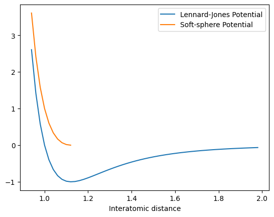

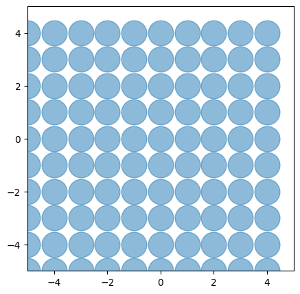
To run a simulation, we will put atoms on a regular grid and draw the velocities from a random distribution with magnitudes corresponding to a specified temperature:

def initcoords(n, l):
    coords = np.zeros((n, 2))
    i = 0
    for x in np.arange(-l[0] / 2, l[0] / 2, l[0] / np.ceil(np.sqrt(n))):
        for y in np.arange(-l[1] / 2, l[1] / 2, l[1] / np.ceil(np.sqrt(n))):
            coords[i] = np.array([x, y])
            i += 1
            if i == n:
                break
    return coords

def initvels(n, temp, seed):
    np.random.seed(seed)
    vels = np.random.random((n, 2)) - np.ones((n, 2)) * 0.5
    vels = (
        vels
        / np.linalg.norm(vels, axis=1)[:, None]
        * np.sqrt(temp * 2 * (1 - 1 / n))
    )
    vels -= np.sum(vels, axis=0) / n
    return vels


def init(n, l, temp, seed):
    step_count = 0
    coors = initcoords(n, l)
    vels = initvels(n, temp, seed)
    accels = np.zeros((n, 2))
    return step_count, coors, vels, accels

n = 100
l = [10,10]
temp = 2
seed = 0
rcut_squared = 2**(1/3)
dt = 0.005

fig, ax = plt.subplots(figsize=(5, 5))

step_count, coors, vels, accels = init(n, l, temp, seed)
trajectory = [coors]
ax.scatter(coors[:, 0], coors[:, 1], s=700, alpha=0.5)
ax.quiver(coors[:,0],coors[:,1],vels[:,0],vels[:,1])
ax.set(xlim=[-l[0] / 2, l[0] / 2], ylim=[-l[1] / 2, l[1] / 2])

[(-5.0, 5.0), (-5.0, 5.0)]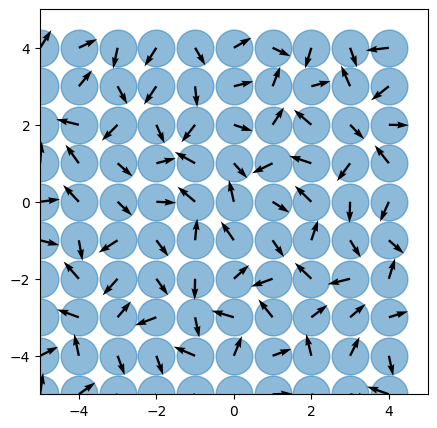

In the above plot, we see the particles in blue, their velocities as black vectors. We now need to write a function for the soft-sphere potential, as well as the negative gradient of it (the force), which can be obtained analytically as

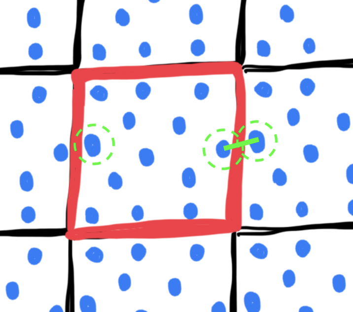
\mathbf{f}_{ij} = -48 \bigl[\bigl(\frac{1}{r_{ij}}\bigr)^{14} - 0.5\bigl(\frac{1}{r_{ij}}\bigr)^{8} \bigr] \mathbf{r}_{ij}

(14)

We will use periodic boundary conditions. That means, instead of making hard boundaries that the particles bounce off of, they can exit the box and re-enter at the same time, similar to a piece of paper you roll up:

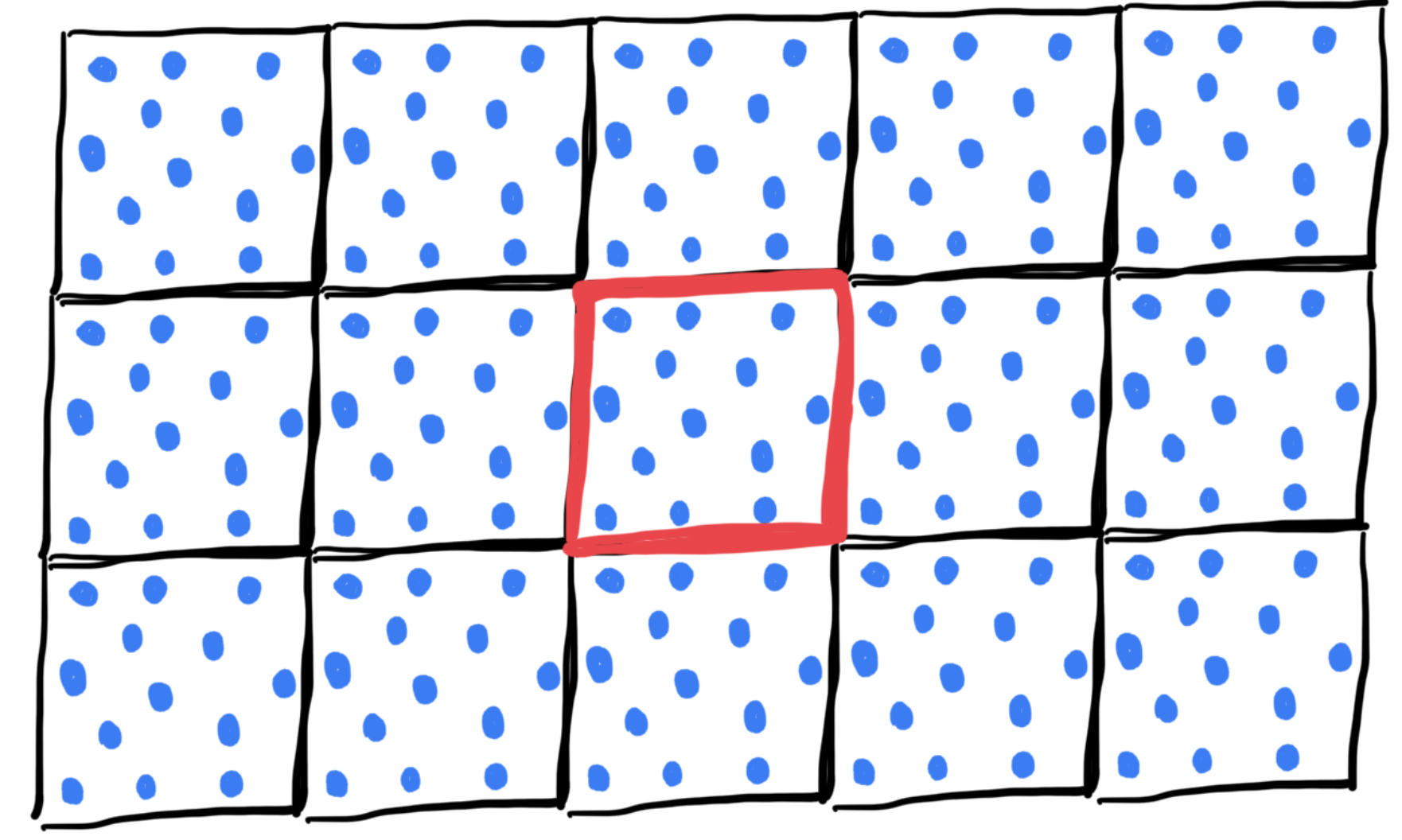
Specifically, this means that for a particle at the other side of the box (on any axis more than half of the box size away):

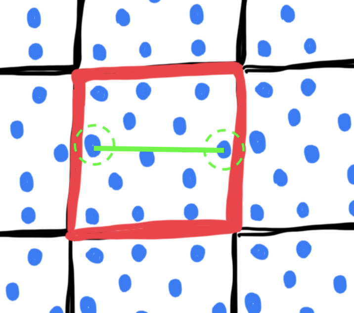
we instead take the “image” of the particle on the other side:

def periodic(coor, l):
    for i in range(2):
        if coor[i] >= 0.5 * l[i]:
            coor[i] -= l[i]
        elif coor[i] < -0.5 * l[i]:
            coor[i] += l[i]
    return coor


def periodic_all(coors, l):
    for i in range(coors.shape[0]):
        coors[i] = periodic(coors[i], l)
    return coors


def soft_sphere(rij_squared):
    rij_squared_inv = 1 / rij_squared
    rij_six_inv = rij_squared_inv**3
    f_val = 48 * rij_six_inv * rij_squared_inv * (rij_six_inv - 0.5)
    e_val = 4 * rij_six_inv * (rij_six_inv - 1) + 1
    return f_val, e_val


def compute_forces(coors, rcut_squared, l):
    n = coors.shape[0]
    accels = np.zeros((n, 2))
    for i in range(n - 1):
        for j in range(i + 1, n):
            vect_rij = periodic(coors[i] - coors[j], l)
            rij_squared = np.sum(vect_rij**2)
            if rij_squared < rcut_squared:
                f_val, e_val = soft_sphere(rij_squared)
                accels[i] += f_val * vect_rij
                accels[j] -= f_val * vect_rij
    return accels

We can now compute forces, and plot them as red arrows (they are currently all zero since the particles are further apart than the cutoff):

accels = compute_forces(coors, rcut_squared, l)

fig, ax = plt.subplots(figsize=(5, 5))
ax.scatter(coors[:, 0], coors[:, 1], s=700, alpha=0.5)
ax.quiver(coors[:,0],coors[:,1],accels[:,0],accels[:,1], color='red')
ax.set(xlim=[-l[0] / 2, l[0] / 2], ylim=[-l[1] / 2, l[1] / 2])

[(-5.0, 5.0), (-5.0, 5.0)]

/opt/conda/lib/python3.12/site-packages/matplotlib/quiver.py:695: RuntimeWarning: divide by zero encountered in scalar divide
  length = a * (widthu_per_lenu / (self.scale * self.width))
/opt/conda/lib/python3.12/site-packages/matplotlib/quiver.py:695: RuntimeWarning: invalid value encountered in multiply
  length = a * (widthu_per_lenu / (self.scale * self.width))

Let us now integrate Newton’s equations of motions, e.g. follow the velocity vector for a very short amount of time to update the positions and then obtain new velocities and forces. We will spend a whole section on integrators, so do not worry about the details here too much, but in principle an integrator works similarly to what is taught at high-school about e.g. throwing a ball: The current position, velocity, and acceleration make up the new position.

def leapfrog_1(r, v, a, dt):
    v_new = v + 0.5*dt*a
    r_new = r + dt*v_new
    return r_new, v_new

def leapfrog_2(v, a, dt):
    v_new = v + 0.5*dt*a
    return v_new

def single_step(coors, vels, accels, rcut_squared, l, dt):
    #step1 leapfrog
    coors, vels = leapfrog_1(coors, vels, accels, dt) 
    coors = periodic_all(coors, l)

    #compute forces
    accels = compute_forces(coors, rcut_squared, l)

    #step2 leapfrog
    vels = leapfrog_2(vels, accels, dt)

    return coors, vels, accels

coors, vels, accels = single_step (coors, vels, accels, rcut_squared, l, dt)
trajectory.append(coors)

fig, ax = plt.subplots(figsize=(5,5))
ax.scatter(coors[:, 0], coors[:, 1], s=700, alpha=0.5)
ax.quiver(coors[:,0],coors[:,1],vels[:,0],vels[:,1])
ax.quiver(coors[:,0],coors[:,1],accels[:,0],accels[:,1], color='red')
ax.set(xlim=[-l[0] / 2, l[0] / 2], ylim=[-l[1] / 2, l[1] / 2])

[(-5.0, 5.0), (-5.0, 5.0)]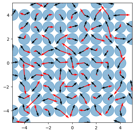

We can see that whereever the spheres of two particles overlap, that there is a strong force away from that overlap. Let us run the simulation for 100 more steps and plot the configuration after the 100 steps:

for i in range(100):
    coors, vels, accels = single_step (coors, vels, accels, rcut_squared, l, dt)
    trajectory.append(coors)
    
fig, ax = plt.subplots(figsize=(5,5))
ax.scatter(coors[:, 0], coors[:, 1], s=700, alpha=0.5)
ax.quiver(coors[:,0],coors[:,1],vels[:,0],vels[:,1])
ax.quiver(coors[:,0],coors[:,1],accels[:,0],accels[:,1], color='red')
ax.set(xlim=[-l[0] / 2, l[0] / 2], ylim=[-l[1] / 2, l[1] / 2])

[(-5.0, 5.0), (-5.0, 5.0)]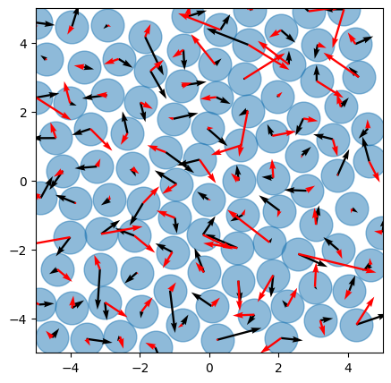

We have now departed from a grid-like structure into a more random, unordered structure. Since the particles cannot leave the box and do not like to overlap, they naturally form a dense packing in 2D, where each particle is roughly surrounded by six other particles.

fig, ax = plt.subplots(figsize=(5, 5))
scat = ax.scatter(trajectory[0][:, 0], trajectory[0][:, 1], s=700, alpha=0.5)
ax.set(xlim=[-l[0] / 2, l[0] / 2], ylim=[-l[1] / 2, l[1] / 2])


def update(frame):
    # for each frame, update the data stored on each artist.
    x = trajectory[frame][:, 0]
    y = trajectory[frame][:, 1]
    # update the scatter plot:
    data = np.stack([x, y]).T
    scat.set_offsets(data)
    return scat


ani = animation.FuncAnimation(fig=fig, func=update, frames=len(trajectory), interval=60)
HTML(ani.to_jshtml())