Numerical integration¶

As the name “molecular dynamics” implies, we will be following the movement/dynamics of atoms and molecules. Conventionally, these movements are created by starting at a specific configuration at time 0, and then integrating Newton’s equations of motion over time. To do so, we need two central pieces of information:

Given the current locations of particles $\mathbf{x}(t)$ and forces $\mathbf{f}$ acting on the atoms, obtain the locations at the next time step $\mathbf{x}(t+1)$
Given the current locations of particles $\mathbf{x}(t)$ , obtain the force $\mathbf{f}(\mathbf{x})$

In this section, we will deal with the first question. It is also known as the N-body problem, and applies to many other fields of research as well, for example to study celestial objects, such as planets moving around a sun. Unfortunately, there is no analytic solution for $N\geq3$ , so that we have to come up with a numeric solution for all but the simplest cases.

import numpy as np
import matplotlib.pyplot as plt

We will start with a case where an analytic solution can be obtained, namely for a single particle (here, a ball) that is thrown from a point $\mathbf{x}(0)$ with a velocity $\mathbf{v}(0)$ and is subject to gravity. Given the initial velocity, angle, gravity (in the y-direction), and heigth (all in SI units), the trajectory is (analytically):

\mathbf{x}(t) = \begin{pmatrix} x_{0} + v_{0,x} \cdot t \\ y_{0} + v_{0,y} \cdot t - \frac{1}{2}gt^2\end{pmatrix}

(1)

def integration_euler(x, v, a, dt):
    new_position = x + dt * v + 0.5 * dt**2 * a
    new_velocity = v + dt * a
    return new_position, new_velocity

def integration_verlet(x, x_1, a, dt):
    new_position = 2*x - x_1 + dt**2 * a
    new_velocity = (new_position - x_1)/(2*dt) 
    return new_position, new_velocity

def integration_leapfrog(x, v_1, a, dt):
    new_velocity = v_1 + dt * a
    new_position = x + dt * new_velocity
    return new_position, new_velocity

def integration_velocity_verlet_positions(x, v, a, dt):
    new_position = x + dt * v + 0.5 * dt**2 * a
    return new_position

def integration_velocity_verlet_velocities(v, a, a__1, dt):
    new_velocity = v + dt * 0.5 * (a + a__1)
    return new_velocity

class ThrowABall:
    def __init__(self, v0, phi, g, y0):
        self.positions = [np.array([0,y0])]
        self.velocities = [np.array([v0*np.cos(phi),v0*np.sin(phi)])]
        self.acceleration = np.array([0, -g])

    def run(self, dt, steps, method='analytic'):
        t = 0
        for _ in range(steps):
            t += dt
            if method == 'analytic':
                new_position = self.positions[0] + self.velocities[0] * t + 0.5 * self.acceleration * t**2
                new_velocity = self.velocities[0] + self.acceleration * t
            elif method == 'euler':
                new_position, new_velocity = integration_euler(self.positions[-1], self.velocities[-1], self.acceleration, dt)
            elif method == 'verlet':
                #not self-starting, we need to estimate the position at t=-1 (!):
                if len(self.positions) == 1:
                    old_position = self.positions[-1] - dt * self.velocities[-1]
                else:
                    old_position = self.positions[-2]
                new_position, new_velocity = integration_verlet(self.positions[-1], old_position, self.acceleration, dt)
            elif method == 'leapfrog':
                #not self-starting, we need to estimate the velocity at t=-0.5 (!):
                if len(self.velocities) == 1:
                    old_velocity = self.velocities[-1] - 0.5 * dt * self.acceleration
                else:
                    old_velocity = self.velocities[-1] # since we work on half steps, this is just the last one
                new_position, new_velocity = integration_leapfrog(self.positions[-1], old_velocity, self.acceleration, dt) 
            elif method == 'velocity_verlet':
                new_position = integration_velocity_verlet_positions(self.positions[-1], self.velocities[-1], self.acceleration, dt)
                new_acceleration = self.acceleration
                new_velocity = integration_velocity_verlet_velocities(self.velocities[-1], self.acceleration, new_acceleration, dt)
            self.positions.append(new_position)
            self.velocities.append(new_velocity)
        return np.array(self.positions)

Since we have the analytic solution, it doesn’t matter whether we choose a small or large time step:

simulation = ThrowABall(5, np.deg2rad(45), 10, 1)
trajectory = simulation.run(0.01, 100)      
plt.scatter(trajectory[:,0], trajectory[:,1], label= 'time step 0.01')

simulation = ThrowABall(5, np.deg2rad(45), 10, 1)
trajectory = simulation.run(0.1, 10)      
plt.scatter(trajectory[:,0], trajectory[:,1], label= 'time step 0.1')

plt.legend()
plt.xlabel("x")
plt.ylabel("y")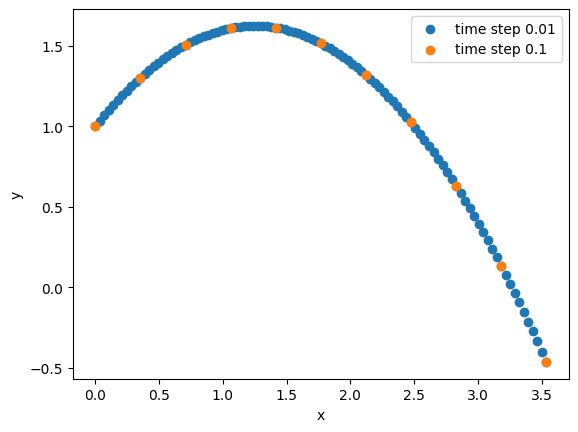

Importantly, we can obtain the solution at any time without any prior knowledge about previous timesteps (apart the initial conditions at time 0), since we have an analytic function of the positions over time. If no analytic function exists, we can integrate the equations of motion numerically. Several m ethods exist, mostly based on Taylor expansions around the current timestep:

\mathbf{x}(t+\Delta t) = \mathbf{x}(t) + \Delta t \cdot \mathbf{v}(t) + \frac{1}{2}\Delta t^2\cdot \mathbf{a}(t) + \frac{1}{6}\Delta t^3\cdot \mathbf{j}(t) + ...

(2)

\mathbf{v}(t+\Delta t) = \mathbf{v}(t) + \Delta t \cdot \mathbf{a}(t) + \frac{1}{2}\Delta t^2\cdot \mathbf{j}(t) + ...

(3)

Euler algorithm¶

The most simple approximation to the complete Taylor expansion would be to simply truncate:

\mathbf{x}(t+\Delta t) = \mathbf{x}(t) + \Delta t \cdot \mathbf{v}(t) + \frac{1}{2}\Delta t^2\cdot \mathbf{a}(t)

(4)

\mathbf{v}(t+\Delta t) = \mathbf{v}(t) + \Delta t \cdot \mathbf{a}(t)

(5)

This algorithm is easy to understand and implement, but not very accurate if the acceleration changes over time (and also not time-reversible). Let’s give it a try:

simulation = ThrowABall(5, np.deg2rad(45), 10, 1)
trajectory = simulation.run(0.1, 10)      
plt.scatter(trajectory[:,0], trajectory[:,1], label= 'analytic')

simulation = ThrowABall(5, np.deg2rad(45), 10, 1)
trajectory = simulation.run(0.1, 10, method='euler')      
plt.scatter(trajectory[:,0], trajectory[:,1], label= 'numeric, Euler')

plt.legend()
plt.xlabel("x")
plt.ylabel("y")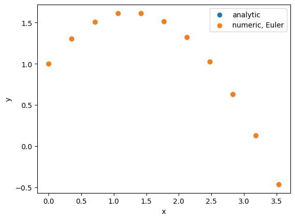

Since the acceleration is constant here, the Euler algorithm gives essentially the same results as the analytic results. We will explore cases where Euler fails later in this notebook. Let us first explore other, more accurate options:

Verlet algorithm¶

Let us revisit the Taylor series, and expand for one step before and after the current time step:

\mathbf{x}(t+\Delta t) = \mathbf{x}(t) + \Delta t \cdot \mathbf{v}(t) + \frac{1}{2}\Delta t^2\cdot \mathbf{a}(t) + \frac{1}{6}\Delta t^3\cdot \mathbf{j}(t) + ...

(6)

\mathbf{x}(t-\Delta t) = \mathbf{x}(t) - \Delta t \cdot \mathbf{v}(t) + \frac{1}{2}\Delta t^2\cdot \mathbf{a}(t) - \frac{1}{6}\Delta t^3\cdot \mathbf{j}(t) + ...

(7)

If we add the two, we get

\mathbf{x}(t+\Delta t) + \mathbf{x}(t-\Delta t) = 2\mathbf{x}(t) + \Delta t^2\cdot \mathbf{a}(t) + ...

(8)

Truncating this after the term for jerk and rearranging gives the formula for the Verlet algorithm:

\mathbf{x}(t+\Delta t) = 2\mathbf{x}(t) - \mathbf{x}(t-\Delta t) + \Delta t^2\cdot \mathbf{a}(t)

(9)

The advantages are again a straightforward implementation. However, there are also several drawbacks. First, the algorithm is not “self-starting”, meaning we have to estimate $\mathbf{x}(-1)$ . Second, adding the small term $\Delta t^2\cdot \mathbf{a}(t)$ to the larger terms $2\mathbf{x}(t) - \mathbf{x}(t-\Delta t)$ causes a loss of numerical precision. Third, there is a lack of an explicit velocity term, which is then usually recovered as $\mathbf{v}(t) = \frac{\mathbf{x}(t+\Delta t) - \mathbf{x}(t-\Delta t)}{2\Delta t}$ .

Let’s give it a try and first estimate $\mathbf{x}(-1) \simeq \mathbf{x}(0) - \Delta t * \mathbf{v}(0)$ :

simulation = ThrowABall(5, np.deg2rad(45), 10, 1)
trajectory = simulation.run(0.1, 10)      
plt.scatter(trajectory[:,0], trajectory[:,1], label= 'analytic')

simulation = ThrowABall(5, np.deg2rad(45), 10, 1)
trajectory = simulation.run(0.1, 10, method='verlet')      
plt.scatter(trajectory[:,0], trajectory[:,1], label= 'numeric, Verlet')

plt.legend()
plt.xlabel("x")
plt.ylabel("y")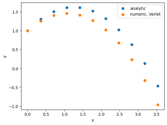

Obviously, this is a terrible result, and is caused by a bad approximation for $\mathbf{x}(-1)$ . Let us make analytic solutions for $\mathbf{x}(0)$ and $\mathbf{x}(1)$ and only start the simulation from there:

simulation = ThrowABall(5, np.deg2rad(45), 10, 1)
trajectory = simulation.run(0.1, 10)      
plt.scatter(trajectory[:,0], trajectory[:,1], label= 'analytic')

simulation = ThrowABall(5, np.deg2rad(45), 10, 1)
trajectory = simulation.run(0.1,1)      
trajectory = simulation.run(0.1,9, method='verlet')      
plt.scatter(trajectory[:,0], trajectory[:,1], label= 'numeric, Verlet')

plt.legend()
plt.xlabel("x")
plt.ylabel("y")

This time, Verlet is again very accurate. Let’s see if we can do better still:

Leapfrog algorithm¶

Let us rearrange the truncated Taylor expansion once more:

\mathbf{x}(t+\Delta t) = \mathbf{x}(t) + \Delta t \cdot \mathbf{v}(t) + \frac{1}{2}\Delta t^2\cdot \mathbf{a}(t) = \mathbf{x}(t) + \Delta t \bigl[ \mathbf{v}(t) + \frac{1}{2}\Delta t\cdot \mathbf{a}(t) \bigr] = \mathbf{x}(t) + \Delta t \cdot \mathbf{v}(t + \frac{1}{2}\Delta t)

(10)

For the velocities, we will subtract the expansions around the half steps:

\mathbf{v}(t+\frac{1}{2}\Delta t) = \mathbf{v}(t) + \frac{1}{2}\Delta t \cdot \mathbf{a}(t)

(11)

\mathbf{v}(t-\frac{1}{2}\Delta t) = \mathbf{v}(t) - \frac{1}{2}\Delta t \cdot \mathbf{a}(t)

(12)

Subtraction gives:

\mathbf{v}(t+\frac{1}{2}\Delta t) - \mathbf{v}(t-\frac{1}{2}\Delta t) = \Delta t \cdot \mathbf{a}(t)

(13)

which rearranges to

\mathbf{v}(t+\frac{1}{2}\Delta t) = \mathbf{v}(t-\frac{1}{2}\Delta t) + \Delta t \cdot \mathbf{a}(t)

(14)

In the leapfrom algorithm, the coordinates and velocities are thus evaluated at different times: We wirst evaluate $\mathbf{v}(t+\frac{1}{2}\Delta t)$ from $\mathbf{v}(t-\frac{1}{2}\Delta t)$ and $\Delta t \cdot \mathbf{a}(t)$ , and then obtain positions at $\mathbf{x}(t+\Delta t)$ from $\mathbf{x}(t)$ and $\mathbf{v}(t + \frac{1}{2}\Delta t)$ .

The advantages are that the Leapfrog algorithm includes a velocity term, that there is no calculation of a difference in large numbers, that it is exactly time-reversible and preserves energy well, and that the implementation is still easy. Disadvantages are that the positions and velocities are not synchronized anymore, and that it is not self-starting.

Let’s give it a try:

simulation = ThrowABall(5, np.deg2rad(45), 10, 1)
trajectory = simulation.run(0.1, 10)      
plt.scatter(trajectory[:,0], trajectory[:,1], label= 'analytic')

simulation = ThrowABall(5, np.deg2rad(45), 10, 1)
trajectory = simulation.run(0.1, 10, method='leapfrog')      
plt.scatter(trajectory[:,0], trajectory[:,1], label= 'numeric, Leapfrog')

plt.legend()
plt.xlabel("x")
plt.ylabel("y")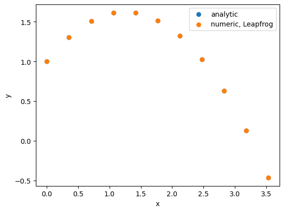

Let’s try to obtain a final algorithm that is also self-starting:

Velocity-Verlet algorithm¶

\mathbf{x}(t+\Delta t) = \mathbf{x}(t) + \Delta t \cdot \mathbf{v}(t) + \frac{1}{2}\Delta t^2\cdot \mathbf{a}(t)

(15)

\mathbf{v}(t+\Delta t) = \mathbf{v}(t) + \Delta t \cdot \frac{\mathbf{a}(t) + \mathbf{a}(t+\Delta t)}{2}

(16)

In practice, this is a three-step procedure where we comput the new positions, then the accelerations at the new positions, and finally the velocity. In our easy case of the ball, the acceleration is constant, so we essentially get the same as Euler. In a general case though, the Velocity-Verlet algorithm has many advantages. It yields synchronized positions and velocities with an explicit velocity term, it is self-starting, there is no calculation of differences of large numbers, and straightforward to implement.

Let’s give it a try:

simulation = ThrowABall(5, np.deg2rad(45), 10, 1)
trajectory = simulation.run(0.1, 10)      
plt.scatter(trajectory[:,0], trajectory[:,1], label= 'analytic')

simulation = ThrowABall(5, np.deg2rad(45), 10, 1)
trajectory = simulation.run(0.1, 10, method='velocity_verlet')      
plt.scatter(trajectory[:,0], trajectory[:,1], label= 'numeric, Velocity-Verlet')

plt.legend()
plt.xlabel("x")
plt.ylabel("y")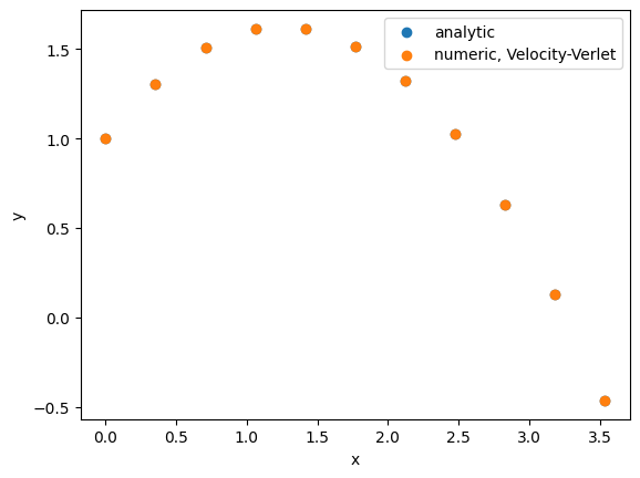

Other integrators¶

There are many other integrations, e.g. Beeman’s algorithm (more accurate expression for velocities but more expensive), or Predictor-Corrector Integration Methods (much more complex and expensive).

Another test-case: Lennard Jones potential:¶

Let us now study a case that is more relevant to chemists, and has an acceleration term that changes over time, so we can better compare the accuracy of the different integrators. We will work with the Lennard-Jones potential, which describes non-bonded interactions of particles, with a weak attraction at longer distances, and a strong repulsion at short distances:

E_\mathrm{pot}(r_{ij}) = 4\epsilon \bigl[\bigl(\frac{\sigma}{r_{ij}}\bigr)^{12} - \bigl(\frac{\sigma}{r_{ij}}\bigr)^{6} \bigr]

(17)

where $\epsilon$ governs the strength of the interaction and $\sigma$ defines the length scale, with the minimum (best) energy at $2^{\frac{1}{6}}\sigma$ . We can analytically take the negative gradient of the potential energy to obtain the force that atom j exerts on atom i:

\mathbf{f}_{ij} = -4\epsilon \bigl[-12\sigma^{12}r_{ij}^{-13} - -6\sigma^6r_{ij}^{-7} \bigr] \frac{\mathbf{r}_{ji}}{r_{ij}} = -\frac{48\epsilon}{\sigma^2} \bigl[\bigl(\frac{\sigma}{r_{ij}}\bigr)^{14} - 0.5\bigl(\frac{\sigma}{r_{ij}}\bigr)^{8} \bigr] \mathbf{r}_{ij}

(18)

In this example, we will work in dimensionless units, where we choose $\sigma$ , $m$ , $\epsilon$ and $\epsilon/k_B$ as units of lenth, masss, energy, and temperature respectively. We thus get the acceleration directly from the force

\mathbf{f}_{ij} = -48 \bigl[\bigl(\frac{1}{r_{ij}}\bigr)^{14} - 0.5\bigl(\frac{1}{r_{ij}}\bigr)^{8} \bigr] \mathbf{r}_{ij}

(19)

(since the conversion factor, namely the mass, is 1).

class TwoAtomsLennardJones:
    def __init__(self, x0, x1):
        self.positions = [np.array([x0,x1])]
        self.velocities = [np.array([[0,0],[0,0]])]
        self.acceleration = []

    def get_a(self, ri, rj):
        vector_rij =  rj - ri
        rij = np.sqrt(vector_rij[0]**2 + vector_rij[1]**2)
        return -48 * (rij**-14 - 0.5 * rij**-8) * vector_rij
        
    def run(self, dt, steps, method='euler'):
        t = 0
        for _ in range(steps):
            t += dt
            self.acceleration.append(np.array([self.get_a(self.positions[-1][0], self.positions[-1][1]),  self.get_a(self.positions[-1][1], self.positions[-1][0])]))
            if method == 'euler':
                new_position, new_velocity = integration_euler(self.positions[-1], self.velocities[-1], self.acceleration[-1], dt)
            elif method == 'verlet':
                #not self-starting, we need to estimate the position at t=-1 (!):
                if len(self.positions) == 1:
                    old_position = self.positions[-1] - dt * self.velocities[-1]
                else:
                    old_position = self.positions[-2]
                new_position, new_velocity = integration_verlet(self.positions[-1], old_position, self.acceleration[-1], dt)
            elif method == 'leapfrog':
                #not self-starting, we need to estimate the velocity at t=-0.5 (!):
                if len(self.velocities) == 1:
                    old_velocity = self.velocities[-1] - 0.5 * dt * self.acceleration[-1]
                else:
                    old_velocity = self.velocities[-1] # since we work on half steps, this is just the last one
                new_position, new_velocity = integration_leapfrog(self.positions[-1], old_velocity, self.acceleration[-1], dt) 
            elif method == 'velocity_verlet':
                new_position = integration_velocity_verlet_positions(self.positions[-1], self.velocities[-1], self.acceleration[-1], dt)
                new_acceleration = np.array([self.get_a(new_position[0], new_position[1]), self.get_a(new_position[1], new_position[0])])
                new_velocity = integration_velocity_verlet_velocities(self.velocities[-1], self.acceleration[-1], new_acceleration, dt)
            self.positions.append(new_position)
            self.velocities.append(new_velocity)
        return np.array(self.positions)

simulation = TwoAtomsLennardJones([0,0],[1.3,0])
trajectory = simulation.run(0.005, 500, method='euler')      
plt.plot(trajectory[:,0,0], label= 'numeric, Euler')


simulation = TwoAtomsLennardJones([0,0],[1.3,0])
trajectory = simulation.run(0.005, 500, method='verlet')      
plt.plot(trajectory[:,0,0], label= 'numeric, Verlet')

simulation = TwoAtomsLennardJones([0,0],[1.3,0])
trajectory = simulation.run(0.005, 500, method='leapfrog')      
plt.plot(trajectory[:,0,0], label= 'numeric, Leapfrog')

simulation = TwoAtomsLennardJones([0,0],[1.3,0])
trajectory = simulation.run(0.005, 500, method='velocity_verlet')      
plt.plot(trajectory[:,0,0],  label= 'numeric, Velocity-Verlet')


plt.legend()
plt.xlabel("steps")
plt.ylabel("x of particle 1")

Starting with atoms slightly further apart than their equilibrium distance, we see that the particles first move closer, until they repell each other, and then oscillate. All integrators apart from Euler are energy-conversing. For the Euler algorithm, we see that small errors accumulate and lead to a complete different behavior (which will eventually lead to the two particles getting separated, and flying apart at a constant velocity):

simulation = TwoAtomsLennardJones([0,0],[1.3,0])
trajectory = simulation.run(0.005, 5000, method='euler')      
plt.plot(trajectory[:,0,0], label= 'numeric, Euler')

simulation = TwoAtomsLennardJones([0,0],[1.3,0])
trajectory = simulation.run(0.005, 5000, method='velocity_verlet')      
plt.plot(trajectory[:,0,0],  label= 'numeric, Velocity-Verlet')

plt.legend()
plt.xlabel("steps")
plt.ylabel("x of particle 1")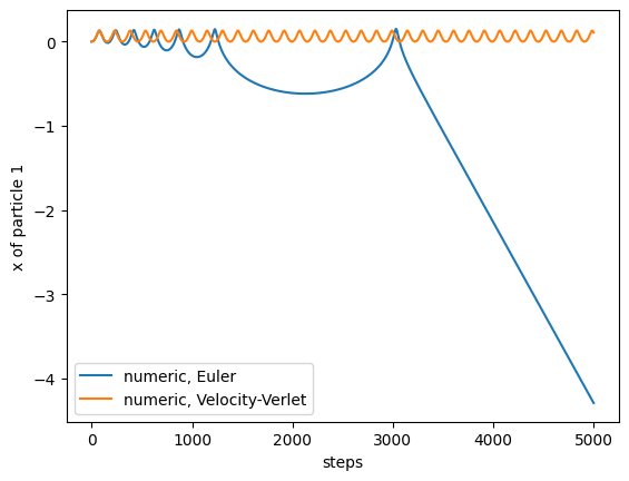

If we wanted to draw any conclusions from this trajectory, we better have not used Euler, otherwise our simulation will be completely unphysical (and useless)!

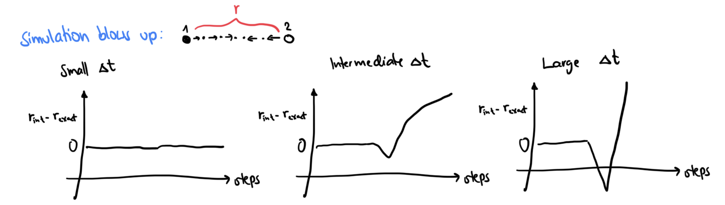
A note on the timestep¶

Another common pitfall is a too large timestep. A (much) too large time step can cause our simulation to blow up. However, there are also more subtle effects before that happens: The numerical accuracy of the numerical integration differs between different methods, and depends on $\Delta t$ .

Inaccuracies cause a drift in the total energies!
For a given potential and system: Make a few short test runs and monitor the energy!