Thermodynamic ensembles¶

Different macroscopic constraints lead to different types of ensembles, with particular statistical characteristics:

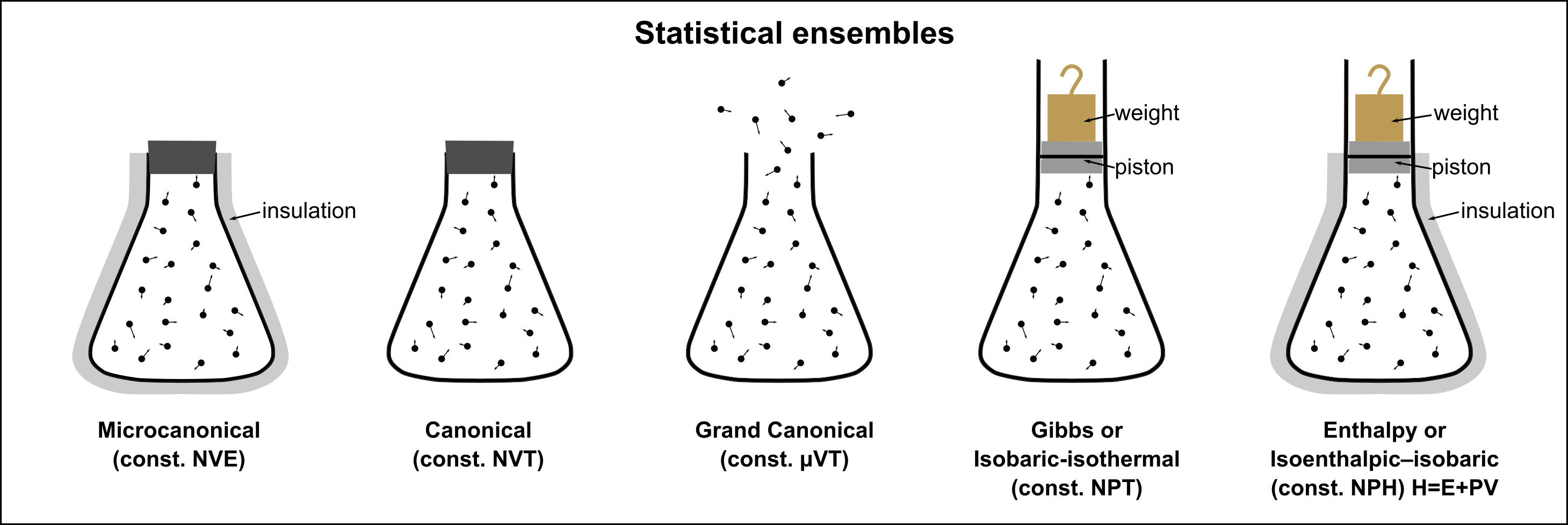
Image by Nzjacobmartin - Own work, CC BY-SA 4.0, https://commons.wikimedia.org/w/index.php?curid=61475757

\textbf{Microcanonical ensemble (or NVE ensemble):} The total energy of the system, its volume and the number of particles in the system are each fixed to particular values.

\textbf{Canonical ensemble (or NVT ensemble):} The energy is not known exactly but the number of particles is fixed. In place of the energy, the temperature $T_0$ is specified. The system is in weak thermal contact with other systems that are described by ensembles with the same temperature (heat bath).

\textbf{Isobaric-isothermal ensemble (or NPT ensemble):} The energy and volume are not known exactly but the number of particles is fixed. In place of the energy, the temperature $T_0$ is specified; in place of the volume, the pressure $P_0$ is specified. The system is in contact with a heat bath, as well as a “pressure bath”.

Thermodynamic results can be transformed between ensembles only for infinitely large systems (in the thermodynamic limit). For finite systems, it is therefore desirably to directly sample in the ensemble of interest:

• Constant temperature: Explore behavior of system as a function of temperature (unfolding of a protein, glass formation), simulated annealing (gradual reduction of the temperature), etc

• Constant temperature and pressure: Modeling of ambient conditions, where the pressure is also constant (which is true for most lab experiments)

What does constant temperature (or pressure) mean?¶

Temperature: On the molecular level, the temperature of a system is defined by the average kinetic energy of all the particles (atoms, molecules) that make up the system.

Statistical mechanical point of view: Impose a temperature on a system by bringing it into thermal contact with a large heat bath.

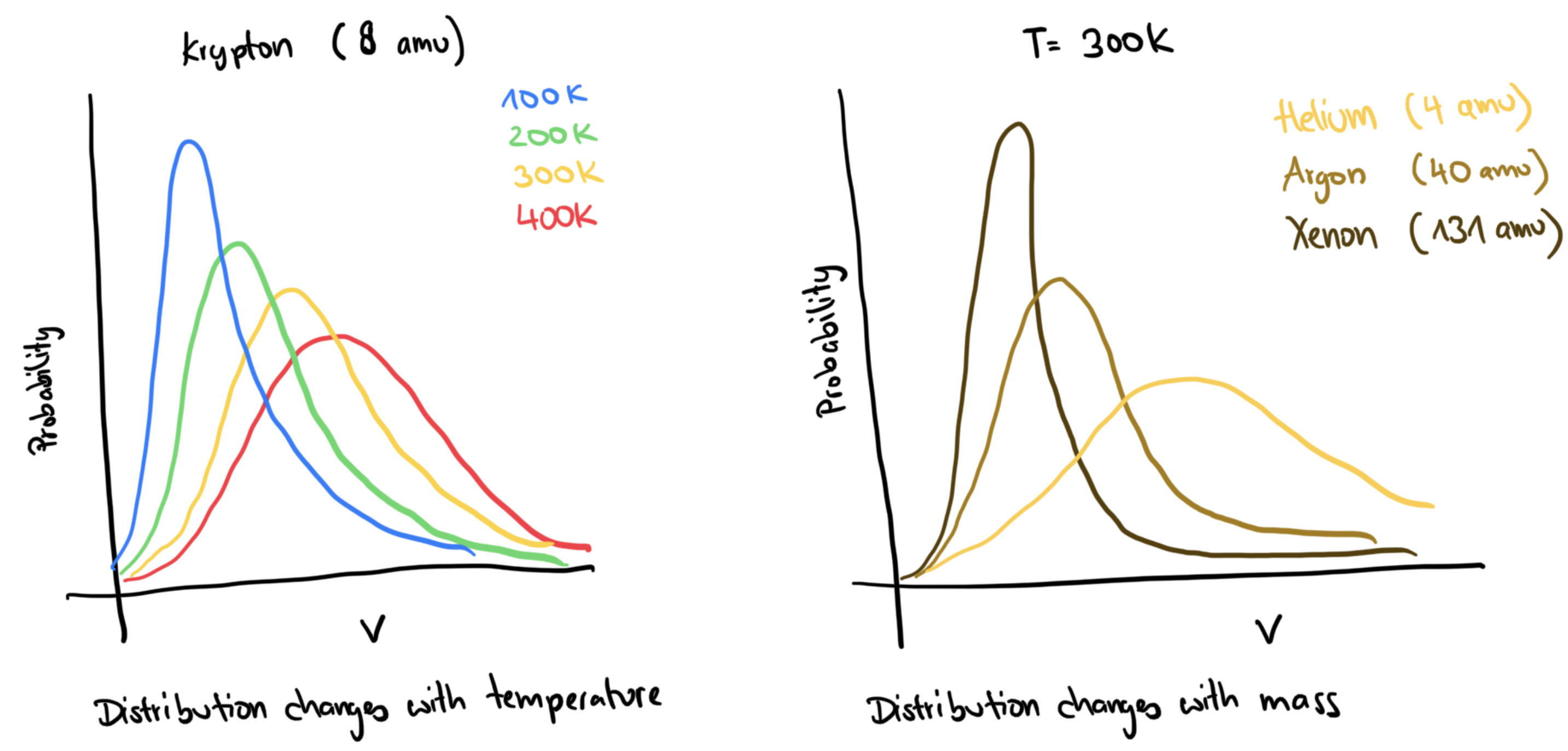
Then, the probability of finding the system in a given energy state is given by the Boltzmann distribution and the velocities are described by the Maxwell-Boltzmann distribution. Thus, the particles won’t all have the same velocity but the velocities will follow a distribution that depends on their mass and the temperature of the system.

Important! Constant temperature $\neq$ kinetic energy per particle is constant

I.e. the relative variance of the kinetic energy per particle in a canonical ensemble is NOT zero, and the instantaneous temperature (obtained via the kinetic energy per particle) fluctuates with a magnitude given by the heat capacity.

Velocity-rescaling (1971)¶

The temperature is related to the total kinetic energy:

To alter the temperature $T(t)$ at timestep $t$, we can therefore scale the velocities by a factor $\lambda$, which yields the change in temperature $\Delta T=T_0-T(t)$:

To change the current temperature to a desired temperature, we can therefore multiply the velocities at each time step by $\lambda= \sqrt{T_0/T(t)}$\[0.5cm]

Advantages

• Simple, easy to understand

• Straightforward to implement

Disadvantages

• Discontinuities in the momentum part of the phase space trajectory

• $T(t)$ cannot fluctuate

• Does not generate rigorous canonical averages

• Artificially prolongs any temperature differences among the components of the system (since only the average temperature is controlled)

Berendsen thermostat (1984)¶

Couple the system to an external heat bath that is fixed to a desired temperature, which supplies or removes heat from the system. At each timestep, scale the velocities such that the rate of temperature change is proportional to the difference in temperature between the bath and the system:

with the coupling parameter $\tau$ (strong coupling for small $\tau$). For one timestep, we therefore get

with the scaling factor

Small $\tau \simeq \Delta t$: Berendsen = velocity-rescaling! Usually: 0.4ps for 1fs timestep ($\tau\simeq 400 \Delta t$)

Advantages

• Simple, easy to understand

• Straightforward to implement

• Much smaller discontinuities in the momentum part of the phase space trajectory than velocity-rescaling

• $T(t)$ can fluctuate (depending on the value of $\tau$)

Disadvantages

• Does not generate rigorous canonical averages

• Artificially prolongs any temperature differences among the components of the system (since only the average temperature is controlled)

Stochastic rescaling (2007)¶

Extension of velocity-rescaling: Reformulate velocity-rescaling in terms of kinetic energy (instead of temperature):

Instead of forcing $E_k(t)$ to be exactly $E_{k,0}$, the target value $E_{k,t}$ is selected stochastically from the canonical equilibrium distribution of the kinetic energy

with $f$ being the nummber of degrees of freedom. The same procedure can be applied to the Berendsen thermostat which yields a smoother trajectory than the formulation above.

Advantages

• Simple, easy to understand

• Straightforward to implement

• Generates correct canonical averages

• $T(t)$ can fluctuate

Disadvantages

• Stochastic, i.e. trajectories cannot be reproduced exactly

Andersen thermostat (1980)¶

Stochastic collisions method where a particle is randomly chosen at intervals and its velocity reassigned by random selection from the Maxwell-Boltzmann distribution.

This is equivalent to a heat bath that randomly emits particles that collide with atoms of the system. Between each collision, the system is simulated with constant energy, so that we obtain a series of short NVE simulations (actually, a Markov chain).\[0.5cm]

The mean rate of collisions $\nu$ determines the strength of the coupling to the heat bath, where successive collisions occur at time intervals of the Poisson distribution

where $P(t,\nu)\mathrm{d}t$ is the probability that the next collision will take place between $t$ and $t+\mathrm{d}t$. For one timestep, the probability of a collision is therefore $\nu\Delta t$. A too low $\nu$ causes the system to not sample from a canonical distribution. A too high $\nu$ leads to too little fluctuations in $T$.

Advantages

• Generates correct canonical averages

Disadvantages

• Dynamic properties cannot be computed correctly, since the dynamics is not physical (randomly decorrelates velocities)

Nos'e-Hoover thermostat (1985)¶

Make the thermal reservoir an integral part of the system by introducing an additional degree of freedom, $s$, with additional, artificial coordinates and velocities. The states of the simulated extended system (coordinates $\mathbf{r}_i$, momenta $\mathbf{p}_i$, time $t$) correspond to the states of the real system ($\mathbf{r}_i'$, $\mathbf{p}_i'$, time $t'$):

Total energy then gets two additional terms:

• Potential energy of the reservoir: $(f+1)k_BT_0\mathrm{ln}s$ where $f$ is the degrees of freedom of the physical system

• Kinetic energy of the reservoir: $\frac{Q}{2}\left( \frac{\mathrm{d}s}{\mathrm{d}t}\right)^2$ with $Q$ being the fictitious mass of the extra degree of freedom ($Q$ therefore influences the strength of the coupling).

We then simulate in the microcanonical ensemble for the extended system (which produces the canonical ensemble in the physical system). The real velocity is $\mathbf{v}_i' = \frac{\mathrm{d}\mathbf{r}_i'}{\mathrm{dt'}} = s\frac{\mathrm{d}\mathbf{r}_i}{\mathrm{dt}}$. We can thus think of the transformation as a timescaling by $\mathrm{d}t' = \mathrm{d}t/s$

Advantages

• Generates correct canonical averages

• One of the most accurate and efficient methods for constant-temperature MD

Disadvantages

• Difficult to understand

• More difficult to implement than other thermostats

• $s$ can change, so that regular time intervals in the extended system correspond to a trajectory of the real system with unevenly spaced time intervals (but there is a method to arrive at evenly spaced intervals). The time evolution of $s$ depends on $Q$.

• Only correct if there is no external force, and the center of mass remains fixed. Possible remedy: A chain of thermostats (Nos'e-Hoover chains with different masses)

• Can exhibit non-ergodic or oscillatory behavior. Possible remedy: A chain of thermostats (Nos'e-Hoover chains with different masses)

Langevin dynamics¶

Temperature is roughly regulated through the addition of friction and random forces (simulates interaction with an artificial solvent) to the equations of motion. The friction coefficient $\gamma$ determines how strong the system is coupled to the heat bath.

• Friction term $m\gamma\mathbf{v}$ removes energy (like the frictional drag of the system moving through a solvent)

• Random term $\mathbf{R}$ adds energy (like collisions/interactions with solvent molecules)

Advantages

• Allows for large timesteps

Disadvantages

• Not deterministic

• Changes dynamics (usually slows down dynamics)

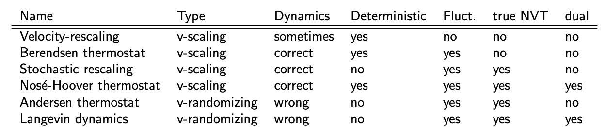
Overview of thermostats¶

The optimal choice of thermostats depends on the properties of interest, as well as the details of the system:

Let us simulate a box of water using the program OpenMM, once with the Langevin thermostat, and once with the Nose-Hover thermostat to showcase this behavior:

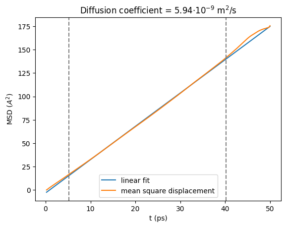
Exercise: Repeat the simulation but choose the “LangevinIntegrator” instead of the “NoseHooverIntegrator”. Use the same settings for temperature, frictionCoeff, and time_step as above. Compute the diffusion coefficient. Do you still get the correct value? Why/why not?

Constant pressure¶

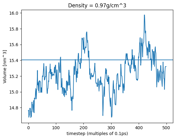
A macroscopic system maintains constant pressure by changing its volume. Similarly, a simulation maintains constant pressure by changing the volume of the simulation cell.

The magnitude of volume fluctuations is related to the isothermal compressibility $\kappa$, where an easily compressible substance undergoes larger pressure fluctuations (similar to the heat capacity being related to energy fluctuations).

Important: The magnitude of volume fluctuations $>>$ magnitude of temperature fluctuations:

• Ideal gas ($\kappa \simeq 1$atm$^{-1}$), simulation in a cube with $L=2$nm ($V=8$nm$^3$) at 300K, the fluctuation in the volume is 18.1nm$^3$ (fluctuation in the cell length of $L=2.6$~nm)! This is therefore not an appropriate simulation size!

• Water ($\kappa \simeq 44.75 10^{-6}$atm$^{-1}$), simulation in a cube with $L=2$nm ($V=8$~nm$^3$) at 300K, the fluctuation in the volume is 0.121nm$^3$ (fluctuation in the cell length of $L=0.49$nm)

Many barostats work very similar to the thermostats already discussed:

• Volume-scaling (not exactly NPT)

• Berendsen-barostat 1984 (not exactly NPT): Coupling to “pressure bath”,

  $$\frac{\mathrm{d}P(t)}{\mathrm{d} t} = \frac{1}{\tau_P}(P_0 - P(t))$$

  (12)

  with the coupling parameter $\tau_P$ (strong coupling for small $\tau_P$), which determines the scaling factor $\lambda$ scaling the volume and thus the atomic coordinates as $\mathbf{r}_i' = \lambda^{1/3}\mathbf{r}_i$

• Stochastic-cell rescaling 2020: Like Berendsen, but additional stochastic term for the rescaling factor that causes the local pressure fluctuations to be correct for the NPT ensemble.

• Andersen 1980/Nos'e-Hoover 1986 barostat: Add extra degree of freedom corresponding to the volume of the box (similar to Nos'e-Hoover thermostat), with potential energy $PV$ and kinetic energy of the piston of $\frac{Q}{2}\left( \frac{\mathrm{d}V}{\mathrm{d}t}\right)^2$ with $Q$ being the fictitious mass of the piston (small mass yields rapid oscillations). The coordinates in the extended system are then related to the real coordinates by $\mathbf{r}_i' = V^{-1/3}\mathbf{r}_i$

• Monte-Carlo barostat 2002: Generate a random volume change from a uniform distribution followed by evaluation of the potential energy of the trial system. The volume move is then accepted with the standard Monte-Carlo probability.

Let us use the MonteCarloBarostat in OpenMM and inspect the volume fluctuations: