Properties¶

Static properties describe measurements of thermodynamic properties, spatial structure and organization

Potential/kinetic energy, heat capacity, pressure, temperature
Radial distribution functions
Number of neighbors
Order

Dynamic properties describe the movements of atoms

Diffusion coefficients
Conductivity
Time-dependent spectroscopy
Viscosity

Let us make another trajectory of our soft-sphere system:

import numpy as np
import matplotlib.pyplot as plt
from scipy.spatial import Voronoi, voronoi_plot_2d
from copy import deepcopy

def periodic(coor, ndim, l):
    for i in range(ndim):
        if coor[i] >= 0.5*l[i]:
            coor[i] -= l[i]
        elif coor[i] < -0.5*l[i]:
            coor[i] += l[i]
    return coor

def periodic_all(coors, n, ndim, l):
    for i in range(n):
        coors[i]=periodic(coors[i], ndim, l)
    return coors

def soft_sphere(rij_squared): 
    rij_squared_inv = 1/rij_squared
    rij_six_inv = rij_squared_inv**3
    f_val = 48 * rij_six_inv * rij_squared_inv * (rij_six_inv - 0.5)
    e_val = 4 * rij_six_inv * (rij_six_inv - 1) + 1
    return f_val, e_val
                
def compute_forces(coors, n, ndim, rcut_squared, l):
    accels = np.zeros((n, ndim))
    sum_pot = 0
    sum_vir = 0
    n_pairs = 0
    for i in range(n-1):
        for j in range(i+1, n):
            n_pairs += 1
            vect_rij = periodic(coors[i]-coors[j], ndim, l)
            rij_squared = np.sum(vect_rij**2)
            if rij_squared < rcut_squared:
                f_val, e_val = soft_sphere(rij_squared)
                accels[i] += f_val * vect_rij
                accels[j] -= f_val * vect_rij
                sum_pot += e_val
                sum_vir += f_val * rij_squared
    return accels, sum_pot, sum_vir, n_pairs

def compute_forces_cell_subdivision(coors, n, ndim, rcut_squared, l, lcell, ncell):
    accels = np.zeros((n, ndim))
    sum_pot = 0
    sum_vir = 0
    cells = np.array((coors+l/2)//lcell,'int')
    cells = [(c[0],c[1]) for c in cells]
    n_pairs = 0
    for mx in range(ncell[0]):
        for my in range(ncell[1]):
            mxp1=int((mx+1)%ncell[0])
            myp1=int((my+1)%ncell[1])
            mym1=int((my-1)%ncell[1])
            cond = [(mxp1, mym1), (mxp1,my), (mxp1,myp1), (mx, myp1)]
            idxs_center = [idx for idx, c in enumerate(cells) if c==(mx,my)]
            idxs_surr = [idx for idx, c in enumerate(cells) if c in cond]
            for ii,i in enumerate(idxs_center):
                for j in idxs_center[ii+1:]+idxs_surr:
                    n_pairs += 1
                    vect_rij = periodic(coors[i]-coors[j], ndim, l)
                    rij_squared = np.sum(vect_rij**2)
                    if rij_squared < rcut_squared:
                        f_val, e_val = soft_sphere(rij_squared)
                        accels[i] += f_val * vect_rij
                        accels[j] -= f_val * vect_rij
                        sum_pot += e_val
                        sum_vir += f_val * rij_squared
    return accels, sum_pot, sum_vir, n_pairs

def compute_forces_neighbor_list(coors, n, ndim, rcut_squared, l, lcell, ncell, refresh, rcut_dr_squared, neighbors):
    accels = np.zeros((n, ndim))
    sum_pot = 0
    sum_vir = 0
    n_pairs = 0
    if refresh:
        cells = np.array((coors+l/2)//lcell,'int')
        cells = [(c[0],c[1]) for c in cells]
        for mx in range(ncell[0]):
            for my in range(ncell[1]):
                mxp1=int((mx+1)%ncell[0])
                myp1=int((my+1)%ncell[1])
                mym1=int((my-1)%ncell[1])
                cond = [(mxp1, mym1), (mxp1,my), (mxp1,myp1), (mx, myp1)]
                idxs_i = [idx for idx, c in enumerate(cells) if c==(mx,my)]
                idxs_j = [idx for idx, c in enumerate(cells) if c in cond]
                for ii,i in enumerate(idxs_i):
                    for j in idxs_i[ii+1:]+idxs_j:
                        n_pairs += 1
                        vect_rij = periodic(coors[i]-coors[j], ndim, l)
                        rij_squared = np.sum(vect_rij**2)
                        if rij_squared < rcut_dr_squared:
                            if i<j:
                                neighbors[i, j] = True
                            else:
                                neighbors[j, i] = True
                        else:
                            if i<j:
                                neighbors[i, j] = False
                            else:
                                neighbors[j, i] = False
                        if rij_squared < rcut_squared:
                            f_val, e_val = soft_sphere(rij_squared)
                            accels[i] += f_val * vect_rij
                            accels[j] -= f_val * vect_rij
                            sum_pot += e_val
                            sum_vir += f_val * rij_squared
        refresh=False
        return accels, sum_pot, sum_vir, n_pairs, neighbors, refresh
        
    for i in range(n-1):
        for j in range(i+1, n):
            if not neighbors[i, j]:
                continue
            n_pairs += 1
            vect_rij = periodic(coors[i]-coors[j], ndim, l)
            rij_squared = np.sum(vect_rij**2)
            if rij_squared < rcut_squared:
                f_val, e_val = soft_sphere(rij_squared)
                accels[i] += f_val * vect_rij
                accels[j] -= f_val * vect_rij
                sum_pot += e_val
                sum_vir += f_val * rij_squared
    return accels, sum_pot, sum_vir, n_pairs, neighbors, refresh

#Use adapted Leapfrog that gives velocities and positions at the same timestep
#The process then becomes 2 steps
def leapfrog_1(r, v, a, dt):
    v_new = v + 0.5*dt*a
    r_new = r + dt*v_new
    return r_new, v_new

def leapfrog_2(v, a, dt):
    v_new = v + 0.5*dt*a
    return v_new

def initcoords(n, ndim, l, ucell):
    coords = np.zeros((n, ndim))
    i=0
    if ndim==2:
        for x in np.arange(-l[0]/2, l[0]/2, l[0]/ucell[0]):
            for y in np.arange(-l[1]/2, l[1]/2, l[1]/ucell[1]):
                coords[i] = np.array([x,y])
                i+=1
                if i == n:
                    break     
    return coords

def initvels(n, ndim, temp, seed):
    np.random.seed(seed) 
    vels = np.random.random((n,ndim))-np.ones((n,ndim))*0.5
    vels = vels/np.linalg.norm(vels, axis=1)[:,None]* np.sqrt(temp*ndim*(1-1/n))
    vels -= np.sum(vels, axis=0)/n
    return vels

def init(n, ndim, l, ucell, temp, seed):
    step_count = 0
    coors = initcoords(n, ndim, l, ucell)
    vels = initvels(n, ndim, temp, seed)
    accels = np.zeros((n, ndim))
    return step_count, coors, vels, accels
            
def single_step(step_count, coors, vels, accels, density, n, ndim, rcut_squared, l, temp, nprint, dt, method, lcell, ncell, refresh, rcut_dr_squared, neighbors):
    #step1 leapfrog
    coors, vels = leapfrog_1(coors, vels, accels, dt) 
    coors = periodic_all(coors, n, ndim, l)

    #compute forces
    if method == 'all_pair':
        accels, sum_pot, sum_vir, n_pairs = compute_forces(coors, n, ndim, rcut_squared, l)
    elif method == 'cell_subdivision':
        accels, sum_pot, sum_vir, n_pairs = compute_forces_cell_subdivision(coors, n, ndim, rcut_squared, l, lcell, ncell)
    elif method == 'neighbor_list':
        accels, sum_pot, sum_vir, n_pairs, neighbors, refresh = compute_forces_neighbor_list(coors, n, ndim, rcut_squared, l, lcell, ncell, refresh, rcut_dr_squared, neighbors)
    else:
        raise NotImplentedError("Unknown method")

    #step2 leapfrog
    vels = leapfrog_2(vels, accels, dt)
    
    kin_energy = 0.5*np.sum(vels**2)/n #per atom
    pot_energy = sum_pot/n #per atom
    tot_energy = kin_energy + pot_energy #per atom
    temp = 2*kin_energy/ndim
    total_vel = np.linalg.norm(np.sum(vels,axis=0))
    pressure = density*(total_vel**2 + sum_vir) / (n*ndim)

    
    if step_count%nprint == 0:
        print("%7i %7.3f %7.3f %7.3f %7.3f %7.3f %7i" % (step_count,
                                               kin_energy,
                                               pot_energy,
                                               tot_energy,
                                               temp,
                                               pressure,
                                               n_pairs))
    step_count += 1
    return step_count, coors, vels, accels, refresh, neighbors

def simulation(ucell, rcut, temp, density, dt, steps, nprint, method, dr=0.3, seed=0):
    n = np.prod(ucell)
    ndim = ucell.shape[0]
    if ndim!=2:
        raise NotImplementedError("Ndim other than 2 not implemented currently")
    l = 1/np.sqrt(density)*ucell
    rcut_squared = rcut**2
    ncell = np.array(np.floor(l/rcut),'int')
    lcell = l/ncell
    refresh = True
    cum_max_vels = 0
    neighbors = np.zeros((n, n), dtype='bool')
    rcut_dr_squared = (rcut+dr)**2
    
    print("%7s %7s %7s %7s %7s %7s %7s" % ("Step", "E_k", "E_pot", "E_tot", "T", "P", "Eval r"))
    traj=[]
    traj_v=[]
    step_count, coors, vels, accels = init(n, ndim, l, ucell, temp, seed)
    for _ in range(steps):
        if cum_max_vels > dr/(2*dt):
            refresh=True
            cum_max_vels = 0
        step_count, coors, vels, accels, refresh, neighbors = single_step(step_count, coors, vels, accels, density, n, ndim, rcut_squared, l, temp, nprint, dt, method, lcell, ncell, refresh, rcut_dr_squared, neighbors)
        cum_max_vels += np.max(np.linalg.norm(vels, axis=1))
        traj.append(coors)
        traj_v.append(vels)
    return traj, traj_v

ucell = np.array([20, 20])
rcut = 2 ** (1 / 6)
temp = 1.0
density = 0.8
dt = 0.001
steps = 5000

ndim = len(ucell)
n = np.prod(ucell)
l = 1 / np.sqrt(density) * ucell

traj, traj_v = simulation(
    ucell,
    rcut,
    temp,
    density,
    dt,
    steps,
    1000,
    "neighbor_list",
)

   Step     E_k   E_pot   E_tot       T       P  Eval r

      0   0.995   0.001   0.996   0.995   0.237    1849

   1000   0.675   0.321   0.996   0.675   3.790    1047

   2000   0.659   0.337   0.996   0.659   3.908    1027

   3000   0.630   0.366   0.996   0.630   4.213    1036

   4000   0.645   0.351   0.996   0.645   4.109    1043

Static properties¶

Static properties can be computed directly from trajectories:

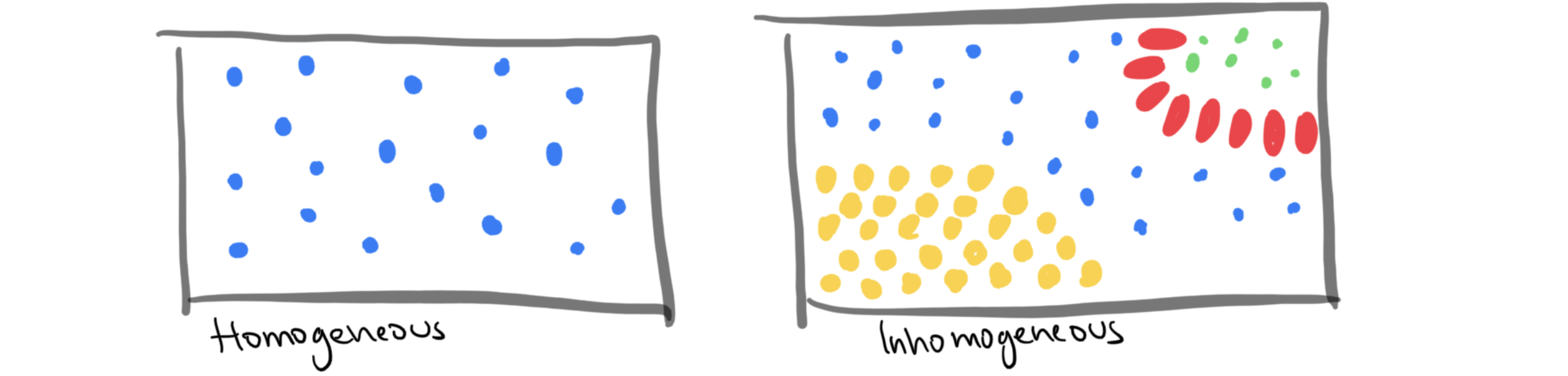
Straightforward: Homogeneous, stationary (equilibrated) systems, where we can average over time and space
Inhomogeneous systems: Localized measurements instead of global averages
Nonstationary over time: No long-term time averaging

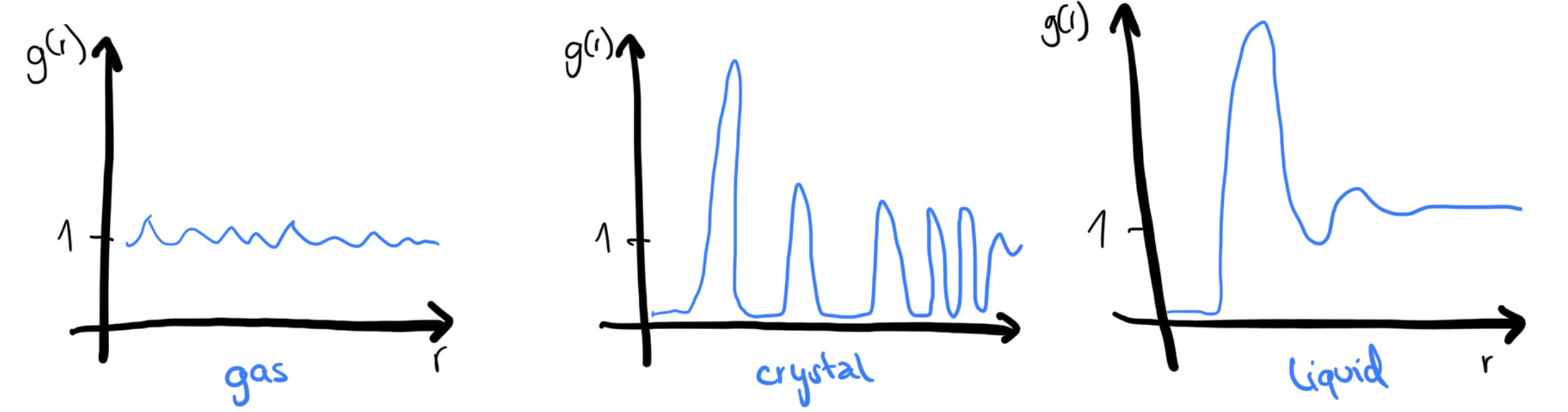
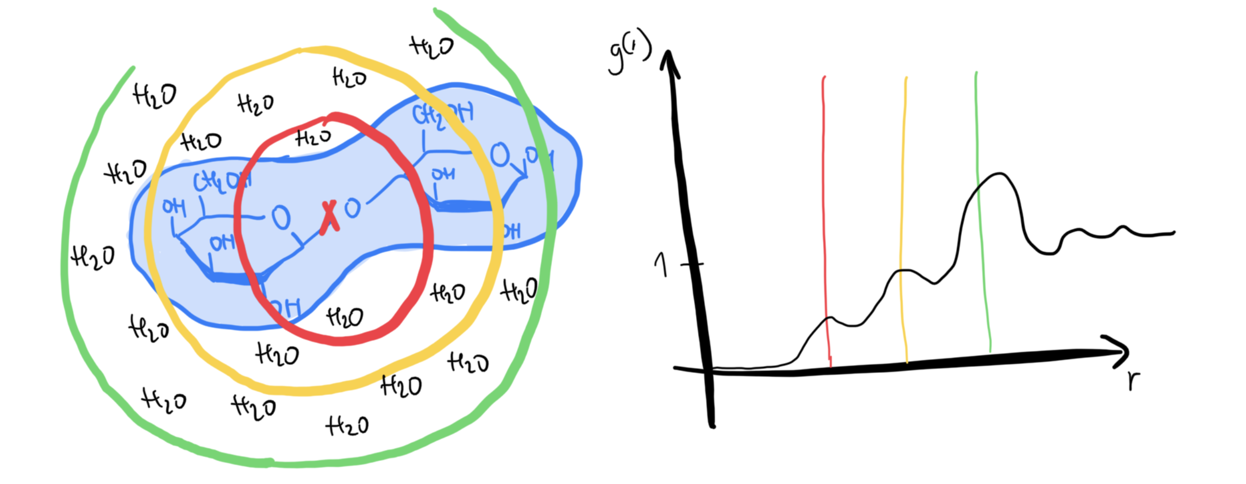
Radial distribution function (pair correlation function) g(r)¶

$g(r)$ describes the spherically averaged local organization around any given atom

$g(r) = \frac{\overline{n}(r)}{\rho V_\mathrm{shell} }$

with $\overline{n}(r)$ the mean number of particles between distance $r$ and $r + \Delta r$ , and $\rho$ the number density $N/V$

It can be derived from a histogram $h_n$ of discretized pair separations, where $\overline{n}(r_n) = h_n*2/N$ , which is the number of atom pairs (i,j) for which $n \Delta r \leq r_{ij} < (n+1)\Delta r$

For small $\Delta r$ :

3 dimensions: $g(r) \simeq \frac{\overline{n}(r)}{4\pi r^2\Delta r \rho}$ with $V_\mathrm{shell} = \frac{4\pi}{3}(r+\Delta r)^3 - \frac{4\pi}{3}r^3 \simeq 4\pi r^ 2\Delta r$
2 dimensions: $g(r) \simeq \frac{\overline{n}(r)}{2\pi r\Delta r \rho}$ with $V_\mathrm{shell} = \pi(r+\Delta r)^2 - \pi r^2 \simeq 2\pi r\Delta r$

Characteristics:

$\rho g(r)d\overrightarrow{r}$ is proportional to the probability of finding an atom in the volume element $d\overrightarrow{r}$ at a distance $r$ from a given atom
$\rho V_\mathrm{shell} \cdot g(r)$ is the mean number of atoms in a shell of radius $r$ and thickness $\Delta r$ surrounding the atom.

Typical behavior:

What is it used for?

central role in liquid-state physics
functions that depend on the pair separation (potential energy, pressure) can be expressed in terms of integrals involving $g(r)$ . E.g. with the pair potential $u(r)$ : $E_\mathrm{pot} = 2\pi N\rho\int_0^\infty r^2 u(r)g(r)dr$
$P = \rho k_b T - \frac{2}{3}\pi\rho^2\int_0^\infty r^3 \frac{du(r)}{dr}g(r)dr$
$g(r)$ is related to the experimentally measurable structure factor $S(\overrightarrow{k})$ ( $\overrightarrow{k}$ is the scattering vector) by Fourier transformation $S(\overrightarrow{k}) = 1+\rho\int g(\overrightarrow{r})e^{-i\overrightarrow{k}\cdot\overrightarrow{r}}d\overrightarrow{r}$ It can therefore be derived experimentally from $S(\overrightarrow{k})$ using neutron scattering or x-ray scattering data
$g(r)$ can even be measured experimentally using microscopy for large particles
$g(r)$ can be used to estimate errors in thermodynamic properties due to the energy cutoff. For example, for the mean potential energy: $\Delta E_\mathrm{pot} = 2\pi \rho \int_{r_c}^\infty r^2u(r)g(r)dr$ Since $g(r)\simeq 1$ for large $r$ , the calculation can be simplified. For the LJ potential, it can even be evaluated analytically: $\Delta E_\mathrm{pot} = 8\pi \rho \left( \frac{1}{9r_c^9}-\frac{1}{3r_c^3} \right)$
Similarly, we can compute the error in the pressure.

Limitations

Radial distribution functions are less meaningful for very asymmetric systems:

def compute_rdf(coords, l, dr=0.1):
    n = len(coords)
    density = n / np.prod(l)
    ndim = len(coords[0])
    rcut = min(l) / 2

    n_bins = int(np.floor(rcut / dr))
    print(rcut, n_bins)
    h = np.zeros(n_bins)
    for i in range(n - 1):
        for j in range(i + 1, n):
            vect_rij = periodic(coords[i] - coords[j], ndim, l)
            rij = np.linalg.norm(vect_rij)
            k = int(rij // dr)
            if k < n_bins:
                h[k] += 1
    r = np.arange(0, n_bins * dr - 0.001, dr)

    if ndim == 3:
        g = h * 2 / n / (density * (4 / 3) * np.pi * ((r + dr) ** 3 - r**3))
    else:
        g = h * 2 / n / (density * np.pi * ((r + dr) ** 2 - r**2))
    return g[1:], r[1:]

i = 0
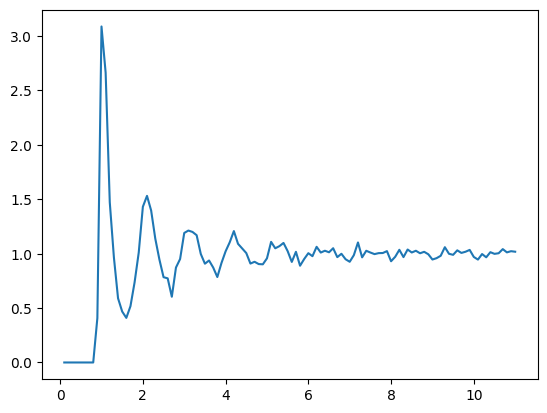
g_r, radii = compute_rdf(traj[i], [22.36067977, 22.36067977])
plt.plot(radii, g_r)

11.180339885 111

i = -1
g_r, radii = compute_rdf(traj[i], [22.36067977, 22.36067977])
plt.plot(radii, g_r)

11.180339885 111

Local order¶

Local order gives information about e.g. how molecules are organized, how large the exposed surface of a large molecule is, etc.

Voronoi subdivision (= tesselation)¶

Construct polyhedra around atoms/molecules such that all points that are closer to a particular atom/molecule than any other belong to its polyhedron. Adjacent atoms/molecules then share a common face of their polyhedra.

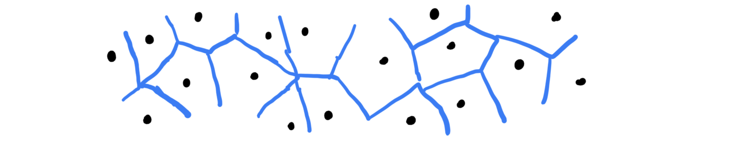
It is commonly used for:

Shape of polyhedra and their volume have a physical meaning
Accurate neighbor counts even for non-spherical molecules
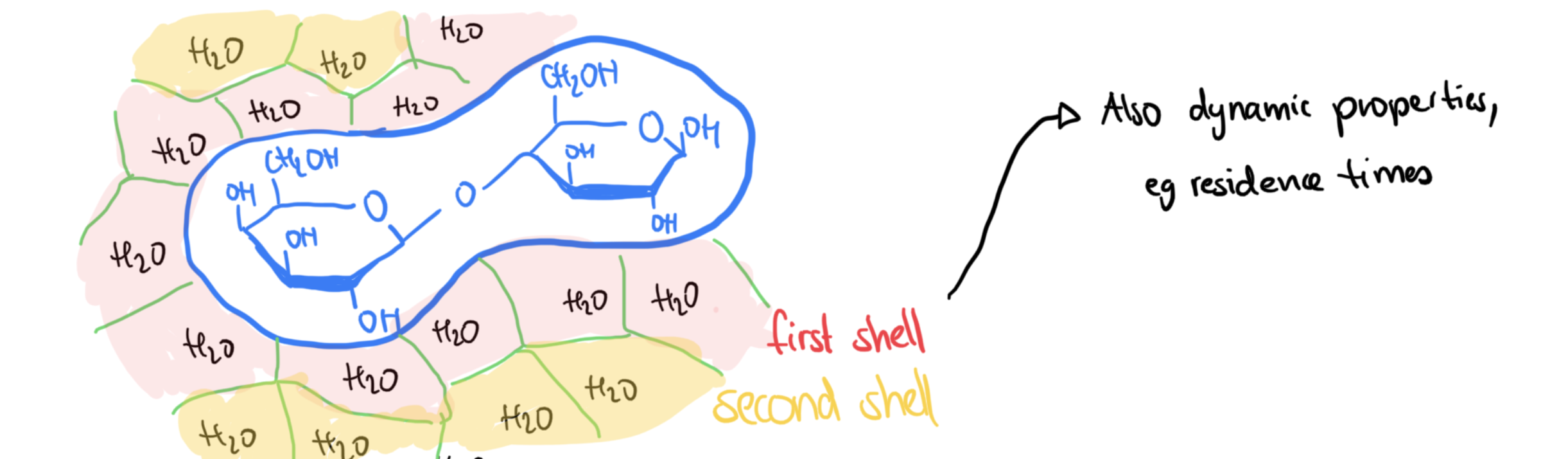
Computation of solvation shells
For mixtures: Number of specific species in the x-th solvation shell

def supercell(coords, L):
    new_points = []
    for i in [-1, 0, 1]:
        for j in [-1, 0, 1]:
            if i == 0 and j == 0:
                continue
            for p in coords:
                if p[0] > L[0] / 2 or p[0] < -L[0] / 2:
                    print(p)
                if p[1] > L[1] / 2 or p[1] < -L[1] / 2:
                    print(p)
                new_points.append(p + np.array([i * L[0], j * L[1]]))
    return np.array(list(coords) + new_points)

l = [22.36067977, 22.36067977]
points = supercell(traj[0], l)

plt.close()
vor = Voronoi(points)
fig = voronoi_plot_2d(vor, show_vertices=False)
plt.xlim([-l[0] / 2, l[0] / 2])
plt.ylim([-l[1] / 2, l[1] / 2])
plt.show()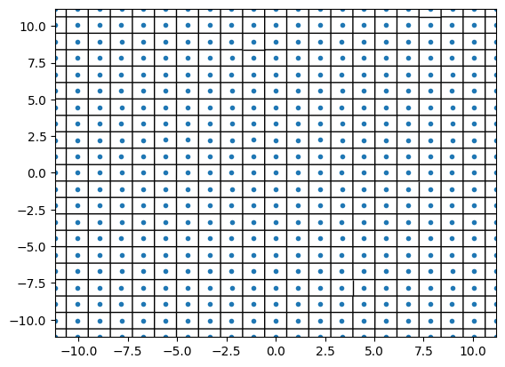

points = supercell(traj[-1], l)

plt.close()
vor = Voronoi(points)
fig = voronoi_plot_2d(vor, show_vertices=False)
plt.xlim([-l[0] / 2, l[0] / 2])
plt.ylim([-l[1] / 2, l[1] / 2])
plt.show()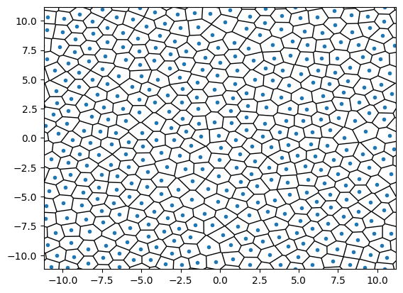

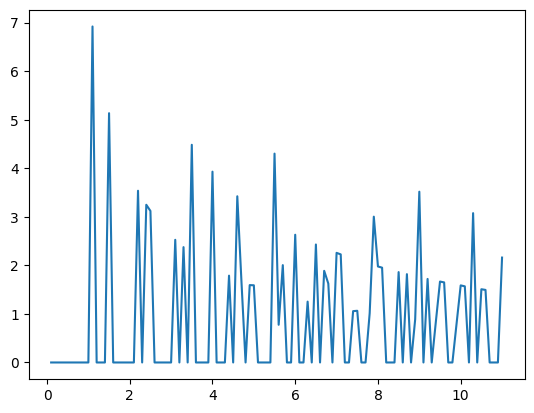
We can easily obtain neighbor counts:

_ = plt.hist([len(x) for x in vor.regions], bins=12)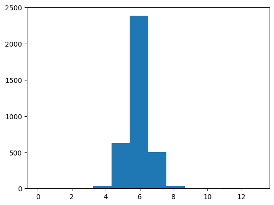

Long-range order¶

$g(r)$ primarily addresses the local structure, and gives only little direct information on long-range (crystalline) order.

The local density at a point $\overrightarrow{r}$ can be expressed as a sum over atoms: $\rho(\overrightarrow{r}) = \sum_j \delta(\overrightarrow{r} - \overrightarrow{r_j})$

Fourier-transforming $\rho(\overrightarrow{r})$ gives $\rho(\overrightarrow{k}) = \frac{1}{N} \sum_j e^{-i\overrightarrow{k} \cdot \overrightarrow{r_j}}$

To test for long-range order, we compute $|\rho(\overrightarrow{k})|$ , and can, for example, follow how a system solidifies.

In our simulation, the long-range order decreases over time, since we start from an ordered system that then gets more and more random:

def compute_lattice(coords, UCELL, L):
    k = np.array(
        [2 * np.pi * 1 * UCELL[0] / L[0], 2 * np.pi * -1 * UCELL[1] / L[1]]
    )
    sr = 0
    si = 0
    for r in coords:
        t = np.dot(r, k)
        sr += np.cos(t)
        si += np.sin(t)
    return np.sqrt(sr**2 + si**2) / len(coords)


plt.close()
x = np.arange(0, 1000, 100)
plt.plot(x, [compute_lattice(traj[i], np.array([20, 20]), l) for i in x])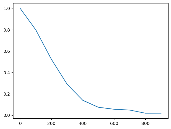

Dynamic properties¶

Dynamic properties are related to nonequilibrium properties. For example, transport coefficients like the diffusion, shear and bulk viscosity, and thermal conductivity arise from mechanical perturbations (concentration, velocity, thermal gradients).

Linear response theory relates the reaction of an equilibrium system to a small external perturbation via equilibrium correlation functions. We can thus compute dynamic properties from equilibrium trajectories.

Namely, the Green-Kubo formalism connects a macroscopic property (=response property of a system) to its equilibrium fluctuations. For example, diffusion is the response to concentration inhomogeneity.

Diffusion coefficient¶

Diffusion coefficients $D$ accessible from the mean-square displacement (\textbf{Einstein expression}): $D = \mathrm{lim}_{t \rightarrow \infty} \frac{\langle \Delta r^2(t) \rangle}{6t} = \mathrm{lim}_{t \rightarrow \infty} \frac{1}{6Nt} \sum_j \Delta r_j ^2$

Derivation:

Fick’s law with $\rho$ ... local density or concentration: $\frac{\partial \rho(\mathbf{r},t)}{\partial t} = D \nabla^2\rho(\mathbf{r},t)$
Multiply by $\Delta r^2$ and integrate along $\mathbf{r}$ : $\frac{\partial}{\partial t} \int \mathrm{d}\mathbf{r} \Delta r^2\rho(\mathbf{r},t) = D \int \mathrm{d}\mathbf{r} \Delta r^2 \nabla^2\rho(\mathbf{r},t)$
Integrate by parts and assume $\rho$ is normalized to 1: \hfill $\frac{\partial}{\partial t} \int \mathrm{d}\mathbf{r} \Delta r^2\rho(\mathbf{r},t) = 2D\cdot d = 6D$
Integral is an expectation value since $\rho$ behaves like a probability: $\frac{\partial}{\partial t} \langle \Delta r^2(t) \rangle = 6D$
$\langle \Delta r^2(t) \rangle$ is linear at long time scales: $\mathrm{lim}_{t \rightarrow \infty} \frac{\langle \Delta r^2(t) \rangle}{t} = 6D$
$\langle \Delta r^2(t) \rangle$ is the average over the particles: $\mathrm{lim}_{t \rightarrow \infty} \frac{\sum_j \Delta r_j(t)^2}{Nt} = 6D$

We thus relate the miscroscopic dynamics ( $\langle \Delta r^2(t) \rangle$ ) with a macroscopic property ( $D$ )

For periodic boundary conditions, we need the true atomic displacements without periodic wraparound (we need to “unfold the trajectory”)!

Unwrapping the trajectory¶

def unwrap(traj, l, ndim):
    new_traj = [traj[0]]
    for i in range(1, len(traj)):
        new = deepcopy(traj[i])
        old = new_traj[i - 1]
        change = new - old
        for ii, p in enumerate(change):
            for j in range(ndim):
                if p[j] >= l[j] / 2:
                    new[ii][j] -= l[j]
                elif p[j] <= -l[j] / 2:
                    new[ii][j] += l[j]
        new_traj.append(new)
    return new_traj

unfolded_traj = unwrap(traj, l, 2)

Diffusion via Einstein expression¶

t0 = 1000
dts = np.arange(0, len(unfolded_traj) - t0, 10)
msd = [
    np.mean(np.sum((unfolded_traj[t0 + t] - unfolded_traj[t0]) ** 2, axis=1))
    for t in dts
]
plt.close()
plt.plot(dts, msd)
plt.show()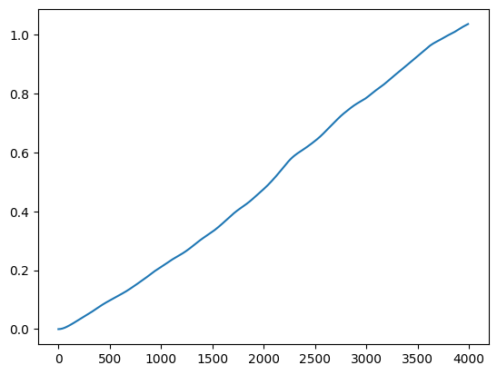

t0 = 1000
t = 3000

np.sum(np.sum((unfolded_traj[t0 + t] - unfolded_traj[t0]) ** 2, axis=1)) / (
    2 * ndim * n * t * dt
)

np.float64(0.06550639059451377)

Diffusion via Velocity Autocorrelation Function (Green-Kubo)¶

Alternative without unfolding: Green-Kubo expression based on the velocity autocorrelation function:

$D = \frac{1}{3}\int_0^\infty \left\langle \mathbf{v}(t) \cdot \mathbf{v}(0)\right\rangle dt$

Derivation:

Start with: \hfill $D = \mathrm{lim}_{t \rightarrow \infty} \frac{1}{6t}\langle \Delta r^2(t) \rangle$
Reformulate $\Delta \mathbf{r}(t)$ as $\int_0^t \mathrm{d}t'\mathbf{v}(t'):$ \hfill $D = \mathrm{lim}_{t \rightarrow \infty} \frac{1}{6t}\int_0^t \mathrm{d}t'\int_0^t \mathrm{d}t''\langle\mathbf{v}(t')\mathbf{v}(t'')\rangle$
One can show that $\int_0^t \mathrm{d}t'\int_0^t \mathrm{d}t''\langle\mathbf{v}(t')\mathbf{v}(t'')\rangle = 2\int_0^\tau \mathrm{d}\tau (t-\tau) \langle\mathbf{v}(\tau)\mathbf{v}(0)\rangle$ , which at $\mathrm{lim}_{t \rightarrow \infty}$ turns into $2t\int_0^\infty \mathrm{d}\tau\langle\mathbf{v}(\tau)\mathbf{v}(0)\rangle$ : \hfill $D = \frac{1}{3}\int_0^\infty \mathrm{d}\tau \langle\mathbf{v}(\tau)\mathbf{v}(0)\rangle$

Important (for Einstein or Green-Kubo relation): For very small box-sizes, we need to include a correction factor!

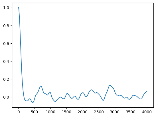
t0 = 1000
t = 4000


norm = sum([np.dot(traj_v[t0][j], traj_v[t0][j]) for j in range(n)])
plt.plot(
    [tt for tt in range(t)],
    [
        sum([np.dot(traj_v[t0 + tt][j], traj_v[t0][j]) for j in range(n)])
        / norm
        for tt in range(t)
    ],
)

t0 = 1000
t = 3000
norm = 1
sum(
    [
        sum([np.dot(traj_v[t0 + tt][j], traj_v[t0][j]) for j in range(n)])
        / norm
        * dt
        for tt in range(t)
    ]
) / (ndim * n)

np.float64(0.09285037676101865)

Shear viscosity¶

The shear viscosity $\eta$ can be obtained via

$\eta = \mathrm{lim}_{t \rightarrow \infty} \frac{1}{6TVt}\left\langle \sum_{x<y} \left[ \sum_j m_j r_{jx}(t)v_{jy}(t) - \sum_j m_j r_{jx}(0)v_{jy}(0)\right]^2\right\rangle$

where $\sum_{x<y}$ denotes a sum over the three pairs of components xy, yz and zx. It characterizes the rate at which some component (e.g. y) of momentum diffuses in a perpendicular (x) direction. This expression is unfortunately unusable with periodic boundary conditions!

Alternative: Green-Kubo expression based on the pressure tensor autocorrelation function:

$\eta = \frac{V}{3T}\int_0^\infty \left\langle \sum_{x<y} P_{xy}(t) P_{xy}(0)\right\rangle dt$ with $P_{xy} = \frac{1}{V}\left[ \sum_j m_jv_{jx}v_{jy} + \frac{1}{2} \sum_{i\neq j} r_{ijx}f_{ijy} \right]$

Thermal conductivity¶

The thermal conductivity $\lambda$ can be obtained via

$\lambda = \mathrm{lim}_{t \rightarrow \infty} \frac{1}{6T^2Vt}\left\langle \sum_{x} \left[ \sum_j r_{jx}(t)e_j(t) - \sum_j r_{jx}(0)e_{j}(0)\right]^2\right\rangle$

where $e_j = \frac{1}{2}mv_j^2 + \frac{1}{2}\sum_{i\neq j} u(r_{ij}) - \langle e \rangle$ is the instantaneous excess energy of atom $j$ , $\langle e \rangle$ is the mean energy and $\sum_{x}$ is a sum over vector components. This expression is unfortunately unusable with periodic boundary conditions!

Alternative: Green-Kubo expression based on the heat flux autocorrelation function:

$\lambda = \frac{V}{3T^2}\int_0^\infty \left\langle \mathbf{S}(t) \mathbf{S}(0)\right\rangle dt$ with $\mathbf{S} = \frac{1}{V}\left[ \sum_j e_j\mathbf{v}_{j} + \frac{1}{2} \sum_{i\neq j} \mathbf{r}_{ij}(\mathbf{f}_{ij}\cdot \mathbf{v}_j)\right]$