Constraints¶

Constraint simulations¶

Conformational behavior of a flexible molecule = complex superpositions of different motions

Translational motion of the center of mass
Rotatiotional motion determined by the torque about the center of mass
Conformational changes and vibrations

Usually: High-frequency motions (e.g. bond vibrations) are of less interest, but they dictate the timestep of the simulation.

C-H bond stretching of hydrocarbons: 2800-3300 cm $^{-1}$

Compute frequency: 90THz = $90\cdot10^{12}$ cycles per second
Period of one cycle: $1\cdot10^{-14}$ s = 10fs
Appropriate timestep: 0.5-1~fs to sample a few points per cycle

Constraint dynamics enables individual, internal coordinates or combinations thereof to be constrained (= fixed) during the simulation without affecting the other degrees if freedom.

Important: Constraint $\neq$ restraint!

Constraint: Bonds or angles are forced to adopt specific values, and the respective degrees of freedom have no energy associated with them.
Restraint: Restrained bonds or angles may deviate from the desired value, the restraint is only an additional term in the forcefield. The respective degree of freedom still has an energy associated with it.

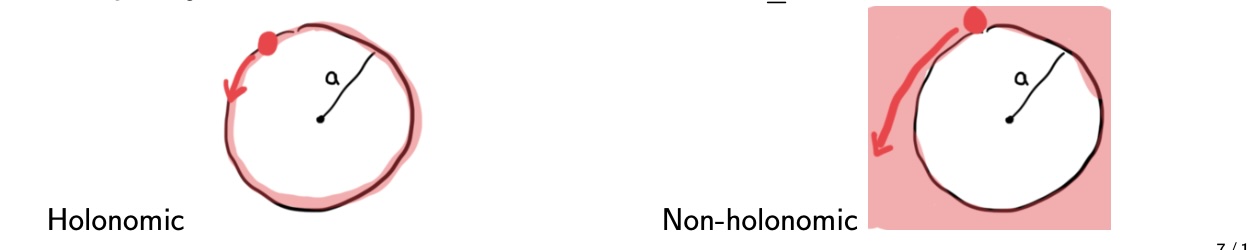
Holonomic vs non-holonomic constraints¶

Holonomic constraints can be expressed in the form

f(q_1, q_2, q_3, ... , t) = 0

(1)

where $q_i$ = coordinates of particle $i$

Example:

Holonomic: Particle with coordinates $r$ is constrained to always lie on the surface of a sphere with radius $a$ , $r^2 - a^2=0$
Non-holonomic Particle with coordinates $r$ can lie on the surface of a sphere with radius $a$ or may fall off, $r^2 - a^2\geq0$

A simple constraint from classical mechanics¶

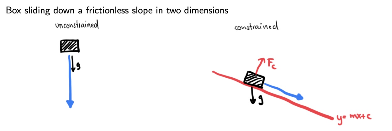
Box is constrained to always remain on the slope, must therefore always satisfy the equation of the slope $y = mx+c$ Without constraint: Box would fall vertically

Gravitational force pulls down along $y$ dimension, but actual motion is along slope. The total force is the sum of a force due to gravity, and due to a constraint force (perpendicular to the surface, does no work since no motion in this direction, i.e. does not change the energy)

Degrees of freedom, and number of coordinates:

Unconstrained system: 3 $N$ degrees of freedom from 3 $N$ independent cartesian coordinates
With $k$ holonomic constraints: 3 $N-k$ degrees of freedom, which can be described using 3 $N-k$ generalized coordinates

E.g. for box: 2 degrees of freedom ( $x$ and $y$ coordinate of box) boils down to a single degree of freedom/generalized coordinate $q$ under constraint of the slope.

Generalized coordinate $q$ along the direction of the slope

Component of the gravitational force along the slope: $Mg\mathrm{sin}\theta$
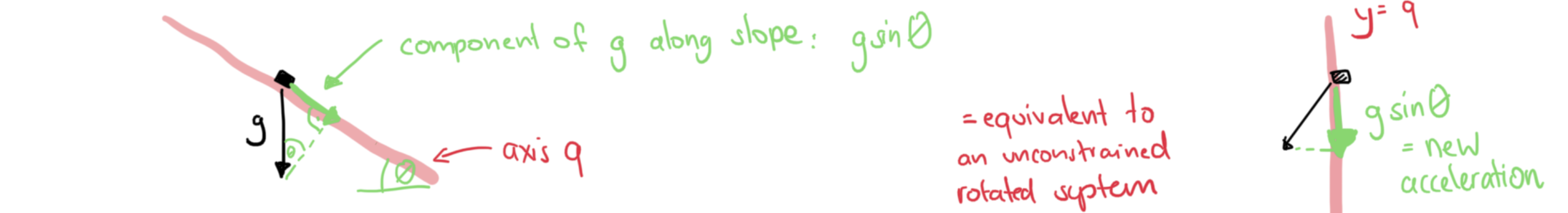
Acceleration down the slope: $g\mathrm{sin}\theta$
Equation of motion:
$\frac{\mathrm{d}^2q}{\mathrm{d}t^2} = g\mathrm{sin}\theta$
(2)
Solution:
$q(t) = q(0) + t \dot{q}(0)+\frac{t^2}{2}g\mathrm{sin}\theta$
(3)

Generalized coordinates can be difficult to find for systems with multiple constraints, it is therefore preferable to work with cartesian coordinates instead:

M \frac{\mathrm{d}^2x}{\mathrm{d}t^2} = F_{cx}

(4)

M \frac{\mathrm{d}^2y}{\mathrm{d}t^2} = -Mg + F_{cy}

(5)

where $F_{cx}$ and $F_{cy}$ are the components of the constraint force.\[0.5cm]

Since the constraint force is perpendicular to the slope, the ratio of the components is given by

\frac{F_{cx}}{F_{cy}} = -m

(6)

We use this by setting $F_{cy}=-\lambda$ , which yields in turn $F_{cx}=\lambda m$ .

We thus get the three equations (two for the equations of motion and one for the constraint):

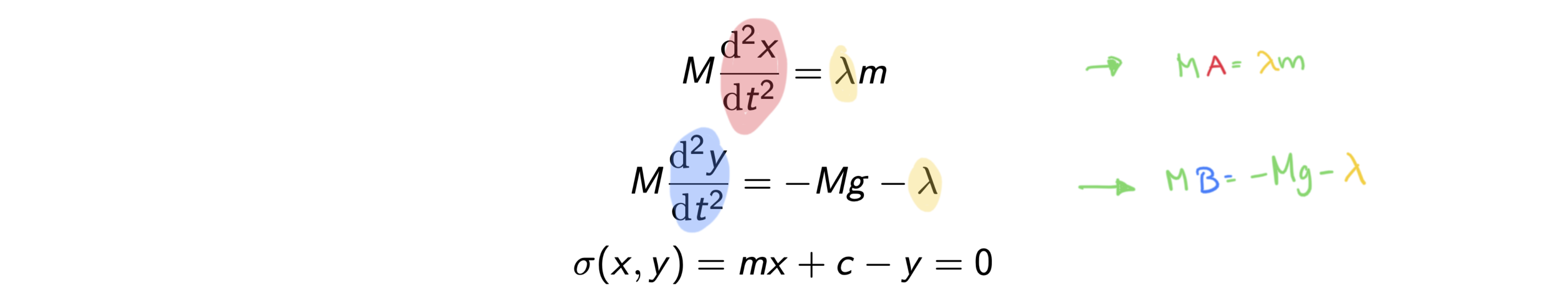
which we can solve using the Lagrange multiplier method. Since $\sigma(x,y)=0$ for all $x,y$ , we can also infer that $\mathrm{d}\sigma = 0$ and $\mathrm{d^2}\sigma = 0$ so that we can reformulate the constraint equation to:

Solving the three equations gives:

\frac{\mathrm{d}^2x}{\mathrm{d}t^2} = -g \frac{m}{1+m^2}

(7)

\frac{\mathrm{d}^2y}{\mathrm{d}t^2} = -g \frac{m^2}{1+m^2}

(8)

which returns the time dependence for $x$ and $y$ :

x(t) = x(0) + t\frac{\mathrm{d}x(0)}{\mathrm{d}t}-g\frac{t^2}{2} \frac{m}{1+m^2}

(9)

y(t) = y(0) + t\frac{\mathrm{d}y(0)}{\mathrm{d}t}-g\frac{t^2}{2} \frac{m^2}{1+m^2}

(10)

Constraints in MD¶

Forces from intra- and intermolecular interactions + forces from constraints

Constraint $\sigma_k$ requires a fixed bond length between atoms $i$ and $j$ :

F_{ckx} = \lambda_k \frac{\partial\sigma_k}{\partial x}

(11)

where $\lambda_k$ is the Lagrange multiplier, $x$ is one of the Cartesian coordinates of the two atoms. The constraint is then

\sigma_{ij} = (\overrightarrow{r}_i-\overrightarrow{r}_j)^2-d_{ij}^2 = 0

(12)

which gives

\frac{\partial\sigma_k}{\partial \overrightarrow{r}_i} = 2(\overrightarrow{r}_i-\overrightarrow{r}_j)

(13)

\frac{\partial\sigma_k}{\partial \overrightarrow{r}_j} = -2(\overrightarrow{r}_i-\overrightarrow{r}_j)

(14)

We can therefore rewrite the forces as (incorporating the factor 2 into $\lambda$ ):

F_{ci} = \lambda (\overrightarrow{r}_i-\overrightarrow{r}_j)

(15)

F_{cj} = -\lambda (\overrightarrow{r}_i-\overrightarrow{r}_j)

(16)

This can be incorporated into the Verlet algorithm:

\overrightarrow{r}_i(t+\Delta t) = 2\overrightarrow{r}_i(t) - \overrightarrow{r}_i(t-\Delta t) + \frac{\Delta t^2}{m_i}\overrightarrow{F}_i(t) + \sum_k\frac{\Delta t^2}{m_i}\lambda_k\overrightarrow{r}_{ij}(t)

(17)

where the summation is over all constraints $k$ that affect atom $i$ . The last term thus perturbs the positions that would have been obtained without constraints.

\overrightarrow{r}_i(t+\Delta t) = \overrightarrow{r}'_i(t+\Delta t) + \sum_k\frac{\Delta t^2}{m_i}\lambda_k\overrightarrow{r}_{ij}(t)

(18)

Determine multipliers $\lambda$ . E.g. for a diatomic molecule:

\overrightarrow{r}_1(t+\Delta t) = \overrightarrow{r}'_1(t+\Delta t) + \frac{\Delta t^2}{m_1}\lambda_{12}(\overrightarrow{r}_{1}(t)-\overrightarrow{r}_{2}(t))

(19)

\overrightarrow{r}_2(t+\Delta t) = \overrightarrow{r}'_2(t+\Delta t) - \frac{\Delta t^2}{m_2}\lambda_{12}(\overrightarrow{r}_{1}(t)-\overrightarrow{r}_{2}(t))

(20)

|\overrightarrow{r}_{1}(t+\Delta t)-\overrightarrow{r}_{2}(t + \Delta t)|^2 = |\overrightarrow{r}_{1}(t)-\overrightarrow{r}_{2}(t)|^2 = d_{12}^2

(21)

Which gives us three equations with three unknown $\overrightarrow{r}_{1}(t+\Delta t)$ , $\overrightarrow{r}_{2}(t+\Delta t)$ , and $\lambda_{12}$ , which can be solved easily.

For many constraints: Solving for Lagrange multipliers becomes equivalent to inverting a $k \times k$ matrix even when we ignore quadratic terms in $\lambda$

Commonly used algorithms are: SHAKE (Ryckaert, Cicotti and Berendsen 1977) Use the above scheme (with the Verlet integrator). Solve each constraint in turn. Since satisfying one constraint might cause the violation of another, it is necessary to iterate around the constraints until they are all satisfied within some tolerance

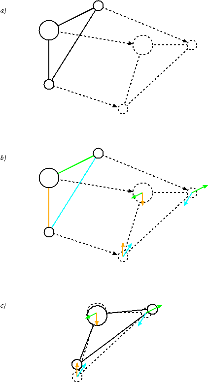By Pedro Gonnet - Own work, CC BY 3.0, https://commons.wikimedia.org/w/index.php?curid=117923908

RATTLE (Andersen 1983) Implementation using Velocity Verlet integrator. This also requires the velocities to be corrected (not only the positions)\[0.5cm]

Many others all differing in how they solve for $\lambda$