Simulation details¶

In this notebook, we will explore tips and tricks to make a simulation both more efficient/fast, as well as accurate. Namely, you will learn

how to compute pair distances efficiently
how to introduce potential cutoffs correctly
how to compute long-ranged interactions with periodic boundary conditions

Efficiency of distance evaluation¶

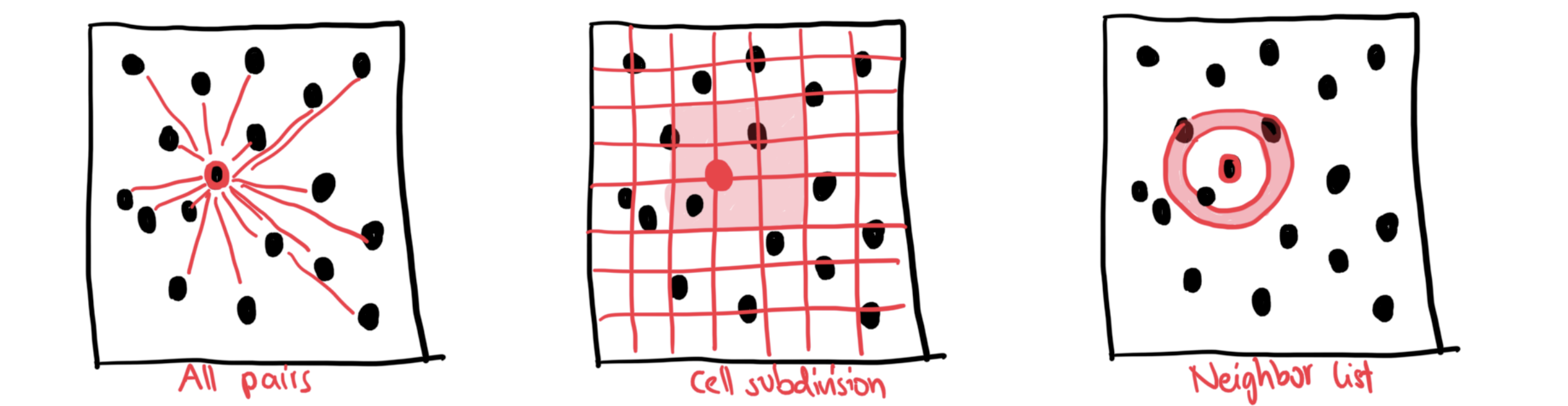
In the last section, we have explored the basics of Newton’s equation of motion ( $\mathbf{f}=m\mathbf{a}$ and $\mathbf{f}=-\nabla E_\mathrm{pot}$ ) to compute our very first simulation of soft spheres. Although our implementation worked, we wasted a lot of computation time. In an MD simulation in general, the computation of the distances between all pairs of particles is often the most time-consuming step. We computed the all-to-all distances of every pair of particles at every time step (which scales with N $^2$ ). Yet, our potential was very short ranged (namely ~1.1 units of length), while our simulation box was 10 units of length, so that particles at opposite sides of the box can surely not interact.

Luckily, there are a few methods available to avoid computing all-to-all distances at every timestep: In cell-subdivision, we only evaluate distances in neighboring cells (red area). In neighbor-lists, we only evaluate distances in a nearby sphere (red area):

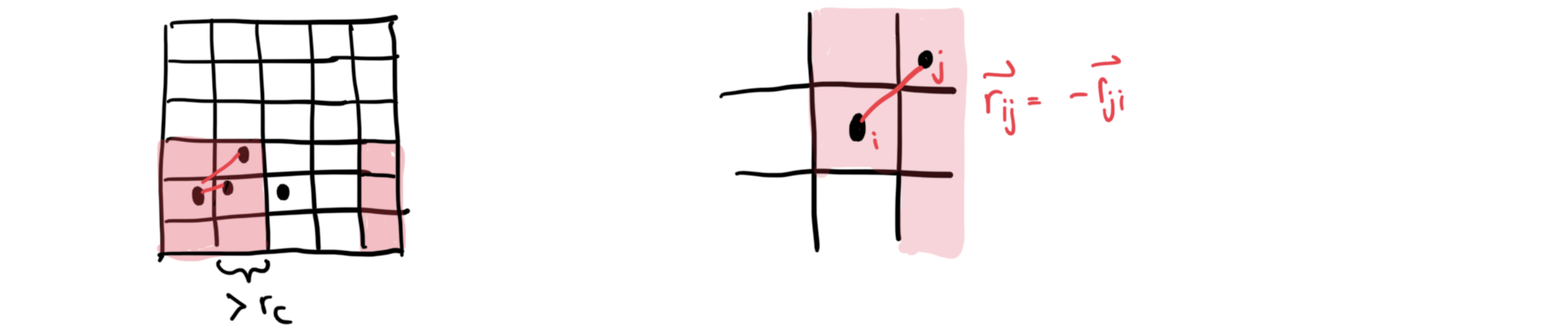
Computing interactions: Cell subdivision¶

Divide simulation region into smaller cells with cell edges $>$ $r_c$
Only atoms in the same or neighboring cells can interact
Due to symmetry ( $r_{ij} = r_{ji})$ , we only need to consider half the neighboring cells
- 3 dimensions: consider 14 neighboring cells
- 2 dimensions: consider 5 neighboring cells
Periodic boundary conditions are easy to include into this scheme

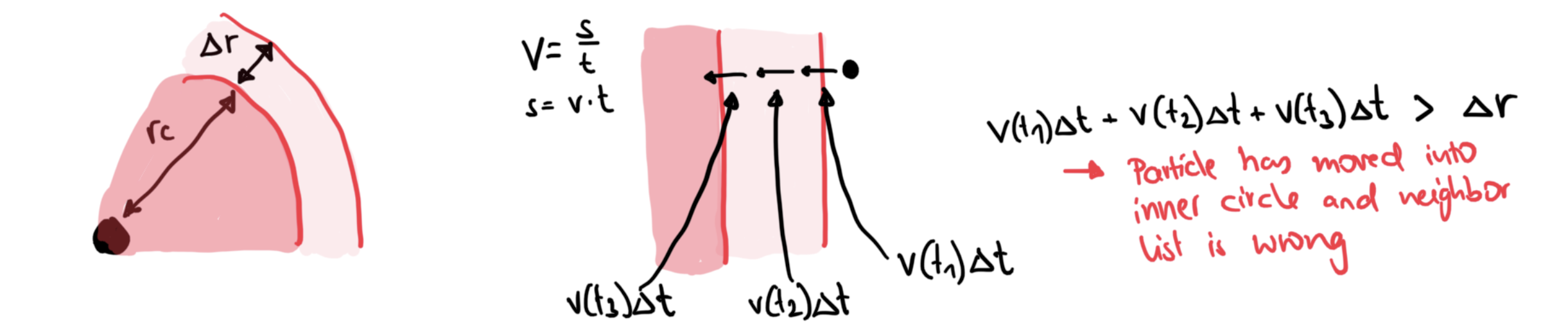
Computing interactions: Neighbor-list method¶

For each atom, keep a list of neighbors at distances $<$ $r_c + \Delta r$
Only atoms in the list can interact
Update list when $\sum_\mathrm{steps}\mathrm{max}v_i > \frac{\Delta r}{2\Delta t}$ (which means that in the next timestep, an atom could have travelled all the way from $r > r_c + \Delta r$ to $r < r_c$
$\Delta r$ is chosen to balance memory requirements, number of distances that need to be computed, and how many times the list needs to be refreshed.
The list refresh can be done with the cell subdivison method

Let us redo our simulation from the last notebook and track the time of the different computation methods.

import numpy as np
import matplotlib.pyplot as plt
import time

def periodic(coor, ndim, l):
    for i in range(ndim):
        if coor[i] >= 0.5*l[i]:
            coor[i] -= l[i]
        elif coor[i] < -0.5*l[i]:
            coor[i] += l[i]
    return coor

def periodic_all(coors, n, ndim, l):
    for i in range(n):
        coors[i]=periodic(coors[i], ndim, l)
    return coors

def soft_sphere(rij_squared): 
    rij_squared_inv = 1/rij_squared
    rij_six_inv = rij_squared_inv**3
    f_val = 48 * rij_six_inv * rij_squared_inv * (rij_six_inv - 0.5)
    e_val = 4 * rij_six_inv * (rij_six_inv - 1) + 1
    return f_val, e_val
                
def compute_forces(coors, n, ndim, rcut_squared, l):
    accels = np.zeros((n, ndim))
    sum_pot = 0
    sum_vir = 0
    n_pairs = 0
    for i in range(n-1):
        for j in range(i+1, n):
            n_pairs += 1
            vect_rij = periodic(coors[i]-coors[j], ndim, l)
            rij_squared = np.sum(vect_rij**2)
            if rij_squared < rcut_squared:
                f_val, e_val = soft_sphere(rij_squared)
                accels[i] += f_val * vect_rij
                accels[j] -= f_val * vect_rij
                sum_pot += e_val
                sum_vir += f_val * rij_squared
    return accels, sum_pot, sum_vir, n_pairs

def compute_forces_cell_subdivision(coors, n, ndim, rcut_squared, l, lcell, ncell):
    accels = np.zeros((n, ndim))
    sum_pot = 0
    sum_vir = 0
    cells = np.array((coors+l/2)//lcell,'int')
    cells = [(c[0],c[1]) for c in cells]
    n_pairs = 0
    for mx in range(ncell[0]):
        for my in range(ncell[1]):
            mxp1=int((mx+1)%ncell[0])
            myp1=int((my+1)%ncell[1])
            mym1=int((my-1)%ncell[1])
            cond = [(mxp1, mym1), (mxp1,my), (mxp1,myp1), (mx, myp1)]
            idxs_center = [idx for idx, c in enumerate(cells) if c==(mx,my)]
            idxs_surr = [idx for idx, c in enumerate(cells) if c in cond]
            for ii,i in enumerate(idxs_center):
                for j in idxs_center[ii+1:]+idxs_surr:
                    n_pairs += 1
                    vect_rij = periodic(coors[i]-coors[j], ndim, l)
                    rij_squared = np.sum(vect_rij**2)
                    if rij_squared < rcut_squared:
                        f_val, e_val = soft_sphere(rij_squared)
                        accels[i] += f_val * vect_rij
                        accels[j] -= f_val * vect_rij
                        sum_pot += e_val
                        sum_vir += f_val * rij_squared
    return accels, sum_pot, sum_vir, n_pairs

def compute_forces_neighbor_list(coors, n, ndim, rcut_squared, l, lcell, ncell, refresh, rcut_dr_squared, neighbors):
    accels = np.zeros((n, ndim))
    sum_pot = 0
    sum_vir = 0
    n_pairs = 0
    if refresh:
        cells = np.array((coors+l/2)//lcell,'int')
        cells = [(c[0],c[1]) for c in cells]
        for mx in range(ncell[0]):
            for my in range(ncell[1]):
                mxp1=int((mx+1)%ncell[0])
                myp1=int((my+1)%ncell[1])
                mym1=int((my-1)%ncell[1])
                cond = [(mxp1, mym1), (mxp1,my), (mxp1,myp1), (mx, myp1)]
                idxs_i = [idx for idx, c in enumerate(cells) if c==(mx,my)]
                idxs_j = [idx for idx, c in enumerate(cells) if c in cond]
                for ii,i in enumerate(idxs_i):
                    for j in idxs_i[ii+1:]+idxs_j:
                        n_pairs += 1
                        vect_rij = periodic(coors[i]-coors[j], ndim, l)
                        rij_squared = np.sum(vect_rij**2)
                        if rij_squared < rcut_dr_squared:
                            if i<j:
                                neighbors[i, j] = True
                            else:
                                neighbors[j, i] = True
                        else:
                            if i<j:
                                neighbors[i, j] = False
                            else:
                                neighbors[j, i] = False
                        if rij_squared < rcut_squared:
                            f_val, e_val = soft_sphere(rij_squared)
                            accels[i] += f_val * vect_rij
                            accels[j] -= f_val * vect_rij
                            sum_pot += e_val
                            sum_vir += f_val * rij_squared
        refresh=False
        return accels, sum_pot, sum_vir, n_pairs, neighbors, refresh
        
    for i in range(n-1):
        for j in range(i+1, n):
            if not neighbors[i, j]:
                continue
            n_pairs += 1
            vect_rij = periodic(coors[i]-coors[j], ndim, l)
            rij_squared = np.sum(vect_rij**2)
            if rij_squared < rcut_squared:
                f_val, e_val = soft_sphere(rij_squared)
                accels[i] += f_val * vect_rij
                accels[j] -= f_val * vect_rij
                sum_pot += e_val
                sum_vir += f_val * rij_squared
    return accels, sum_pot, sum_vir, n_pairs, neighbors, refresh

#Use adapted Leapfrog that gives velocities and positions at the same timestep
#The process then becomes 2 steps
def leapfrog_1(r, v, a, dt):
    v_new = v + 0.5*dt*a
    r_new = r + dt*v_new
    return r_new, v_new

def leapfrog_2(v, a, dt):
    v_new = v + 0.5*dt*a
    return v_new

def initcoords(n, ndim, l, ucell):
    coords = np.zeros((n, ndim))
    i=0
    if ndim==2:
        for x in np.arange(-l[0]/2, l[0]/2, l[0]/ucell[0]):
            for y in np.arange(-l[1]/2, l[1]/2, l[1]/ucell[1]):
                coords[i] = np.array([x,y])
                i+=1
                if i == n:
                    break     
    return coords

def initvels(n, ndim, temp, seed):
    np.random.seed(seed) 
    vels = np.random.random((n,ndim))-np.ones((n,ndim))*0.5
    vels = vels/np.linalg.norm(vels, axis=1)[:,None]* np.sqrt(temp*ndim*(1-1/n))
    vels -= np.sum(vels, axis=0)/n
    return vels

def init(n, ndim, l, ucell, temp, seed):
    step_count = 0
    coors = initcoords(n, ndim, l, ucell)
    vels = initvels(n, ndim, temp, seed)
    accels = np.zeros((n, ndim))
    return step_count, coors, vels, accels
            
def single_step(step_count, coors, vels, accels, density, n, ndim, rcut_squared, l, temp, nprint, dt, method, lcell, ncell, refresh, rcut_dr_squared, neighbors):
    #step1 leapfrog
    coors, vels = leapfrog_1(coors, vels, accels, dt) 
    coors = periodic_all(coors, n, ndim, l)

    #compute forces
    if method == 'all_pair':
        accels, sum_pot, sum_vir, n_pairs = compute_forces(coors, n, ndim, rcut_squared, l)
    elif method == 'cell_subdivision':
        accels, sum_pot, sum_vir, n_pairs = compute_forces_cell_subdivision(coors, n, ndim, rcut_squared, l, lcell, ncell)
    elif method == 'neighbor_list':
        accels, sum_pot, sum_vir, n_pairs, neighbors, refresh = compute_forces_neighbor_list(coors, n, ndim, rcut_squared, l, lcell, ncell, refresh, rcut_dr_squared, neighbors)
    else:
        raise NotImplentedError("Unknown method")

    #step2 leapfrog
    vels = leapfrog_2(vels, accels, dt)
    
    kin_energy = 0.5*np.sum(vels**2)/n #per atom
    pot_energy = sum_pot/n #per atom
    tot_energy = kin_energy + pot_energy #per atom
    temp = 2*kin_energy/ndim
    total_vel = np.linalg.norm(np.sum(vels,axis=0))
    pressure = density*(total_vel**2 + sum_vir) / (n*ndim)

    
    if step_count%nprint == 0:
        print("%7i %7.3f %7.3f %7.3f %7.3f %7.3f %7i" % (step_count,
                                               kin_energy,
                                               pot_energy,
                                               tot_energy,
                                               temp,
                                               pressure,
                                               n_pairs))
    step_count += 1
    return step_count, coors, vels, accels, refresh, neighbors

def simulation(ucell, rcut, temp, density, dt, steps, nprint, method, dr=0.3, seed=0):
    n = np.prod(ucell)
    ndim = ucell.shape[0]
    if ndim!=2:
        raise NotImplementedError("Ndim other than 2 not implemented currently")
    l = 1/np.sqrt(density)*ucell
    rcut_squared = rcut**2
    ncell = np.array(np.floor(l/rcut),'int')
    lcell = l/ncell
    refresh = True
    cum_max_vels = 0
    neighbors = np.zeros((n, n), dtype='bool')
    rcut_dr_squared = (rcut+dr)**2
    
    print("%7s %7s %7s %7s %7s %7s %7s" % ("Step", "E_k", "E_pot", "E_tot", "T", "P", "Eval r"))
    traj=[]
    traj_v=[]
    step_count, coors, vels, accels = init(n, ndim, l, ucell, temp, seed)
    for _ in range(steps):
        if cum_max_vels > dr/(2*dt):
            refresh=True
            cum_max_vels = 0
        step_count, coors, vels, accels, refresh, neighbors = single_step(step_count, coors, vels, accels, density, n, ndim, rcut_squared, l, temp, nprint, dt, method, lcell, ncell, refresh, rcut_dr_squared, neighbors)
        cum_max_vels += np.max(np.linalg.norm(vels, axis=1))
        traj.append(coors)
        traj_v.append(vels)
    return traj, traj_v

times={}
for method in ['all_pair','cell_subdivision','neighbor_list']:
    times[method]=[]
    for NN in [5, 10, 15]:
        start = time.time()
        traj, traj_v = simulation(ucell = np.array([NN,NN]), 
                              rcut = 2**(1/6), 
                              temp = 1.0, 
                              density = 0.8, 
                              dt = 0.005, 
                              steps =100,
                              nprint = 50,
                              method = method)
        end = time.time()
        times[method].append(end-start)

for method in ['all_pair','cell_subdivision','neighbor_list']:
    plt.plot([x**2 for x in [5, 10, 15]], times[method], label=method)

plt.xlabel("Particles")
plt.ylabel("Time")
plt.legend()

   Step     E_k   E_pot   E_tot       T       P  Eval r
      0   0.873   0.003   0.877   0.873   0.303     300

     50   0.613   0.264   0.877   0.613   3.281     300

   Step     E_k   E_pot   E_tot       T       P  Eval r

      0   0.981   0.003   0.985   0.981   0.299    4950

     50   0.646   0.339   0.985   0.646   4.008    4950

   Step     E_k   E_pot   E_tot       T       P  Eval r

      0   0.990   0.004   0.994   0.990   0.315   25200

     50   0.686   0.308   0.994   0.686   3.713   25200

   Step     E_k   E_pot   E_tot       T       P  Eval r
      0   0.873   0.003   0.877   0.873   0.303     168
     50   0.613   0.264   0.877   0.613   3.281     168
   Step     E_k   E_pot   E_tot       T       P  Eval r
      0   0.981   0.003   0.985   0.981   0.299     528

     50   0.646   0.339   0.985   0.646   4.008     512

   Step     E_k   E_pot   E_tot       T       P  Eval r
      0   0.990   0.004   0.994   0.990   0.315    1088

     50   0.686   0.308   0.994   0.686   3.713    1069

   Step     E_k   E_pot   E_tot       T       P  Eval r
      0   0.873   0.003   0.877   0.873   0.303     168
     50   0.613   0.264   0.877   0.613   3.281      60
   Step     E_k   E_pot   E_tot       T       P  Eval r
      0   0.981   0.003   0.985   0.981   0.299     528

     50   0.646   0.339   0.985   0.646   4.008     226
   Step     E_k   E_pot   E_tot       T       P  Eval r
      0   0.990   0.004   0.994   0.990   0.315    1088

     50   0.686   0.308   0.994   0.686   3.713     512

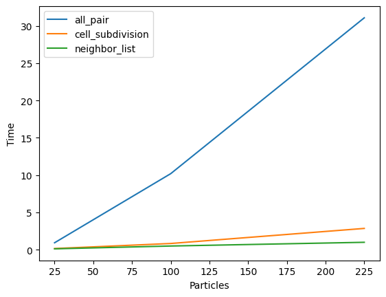
We can see that an all-pair distance evaluation very quickly takes a long time (y-axis) to compute with an increasing number of particles (x-axis)! Note that neiter cell-subdivision, nor neighbor-list are an approximation (!); they are exact, since all interactions beyond our potential cutoff are exactly zero.

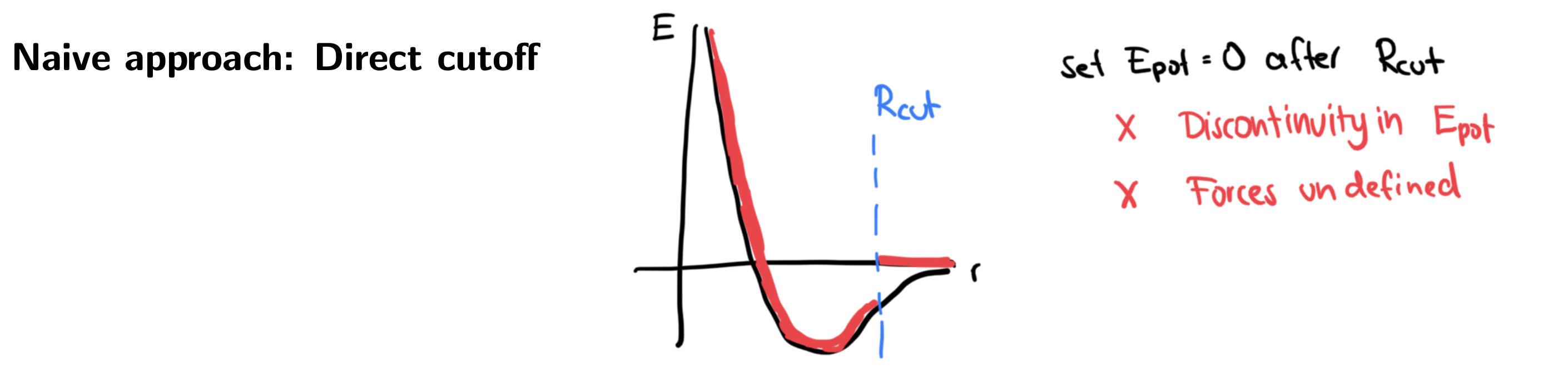
Potential cutoffs¶

This brings us to an important next point: In the soft-sphere potential used above, we had a natural, direct cutoff built into the potential. This is usually not the case, since most potentials

Decay quickly with $R$ (short sighted)
But have a non-zero value for any finite $R$ (non-bounded support)

We have already seen how computing all $R_{IJ}$ in a simulation is computationally expensive. Further, for periodic boundary conditions, we will count atoms multiple times if we do not limit $R_{IJ}$ to a maximum value (smaller than half of the shortest box length). We therefore have to introduce a cutoff function:

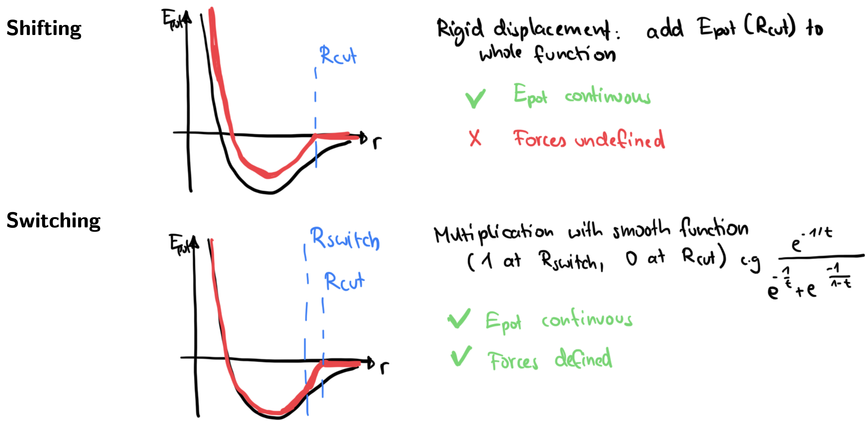
In practice, “switching” is always preferred, and you will find it implemented in any common MD code!

def switch(rij, r_switch, r_cut):
    s = np.zeros_like(rij)
    mask1 = rij <= r_switch
    s[mask1] = 1.0
    mask2 = (rij > r_switch) & (rij < r_cut)
    x = (rij[mask2] - r_switch) / (r_cut - r_switch)
    s[mask2] = np.exp(-1.0 / (1.0 - x)) / (np.exp(-1.0 / x) + np.exp(-1.0 / (1.0 - x)))
    return s

x = np.arange(1, 2.0, 0.001)
plt.plot(x, switch(x, 1.4, 1.6))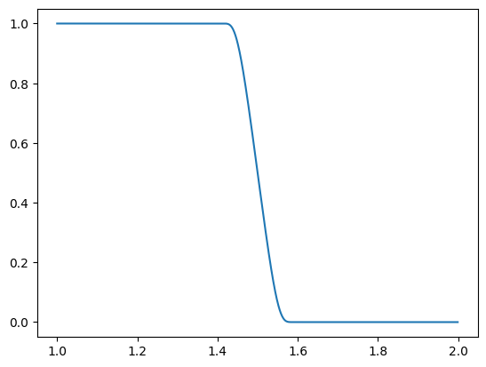

Let us plot how a Lennard Jones potential looks with a cutoff:

def lennard_jones_potential(rij):
    return 4 * (rij ** (-12) - rij ** (-6))

def lennard_jones_potential_cutoff(rij, c):
    return (rij<c)* (4 * (rij ** (-12) - rij ** (-6)))

def lennard_jones_potential_shifting(rij, c):
    return (rij<c)* (4 * (rij ** (-12) - rij ** (-6)) - 4 * (c ** (-12) - c ** (-6))) 
    
def lennard_jones_potential_switching(rij, c1, c2):
    return (4 * (rij ** (-12) - rij ** (-6)) ) * switch(rij, c1, c2)

    
x = np.arange(0.94, 2.0, 0.001)
plt.plot(x, lennard_jones_potential(x), label="LJ potential, no cutoff")
plt.plot(x, lennard_jones_potential_cutoff(x, 1.4), label="LJ potential, direct cutoff")
plt.plot(x, lennard_jones_potential_shifting(x, 1.4), label="LJ potential, shifting")
plt.plot(x, lennard_jones_potential_switching(x, 1.3, 1.4), label="LJ potential, switching")

plt.legend()
plt.xlabel("Potential energy")
plt.xlabel("Interatomic distance")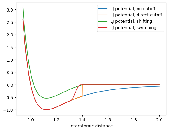

Of course, this plot is very exagerated (with a very small cutoff). In reality, our cutoff would be at much larger distances:

x = np.arange(0.94, 10.0, 0.001)
plt.plot(x, lennard_jones_potential(x), label="LJ potential, no cutoff")
plt.plot(x, lennard_jones_potential_cutoff(x, 8), label="LJ potential, direct cutoff")
plt.plot(x, lennard_jones_potential_shifting(x, 8), label="LJ potential, shifting")
plt.plot(x, lennard_jones_potential_switching(x, 8, 8.5), label="LJ potential, switching")

plt.legend()
plt.xlabel("Potential energy")
plt.xlabel("Interatomic distance")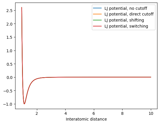

Here, the differences in the potential become negligible, but the downsides (discontinuities for direct cutoff and shifting), of course remain, so that switching is always preferable. It is important that by using a cutoff, we make an approximation, i.e. set all interactions to zero at a certain distance! For a Lennard-Jones potential, this is usually a good approximation since the potential decays quickly. But what about charged interactions? They follow a Coulomb potential which is very long-ranged, since it decays with 1/ $R$ instead of 1/ $R^12$ . For example, for two positively charged particles:

def coulomb_potential(rij):
    return -1 / rij 

plt.plot(x, lennard_jones_potential(x), label="LJ potential, no cutoff")
plt.plot(x, coulomb_potential(x), label="Coulomb potential, no cutoff")

plt.legend()
plt.xlabel("Potential energy")
plt.xlabel("Interatomic distance")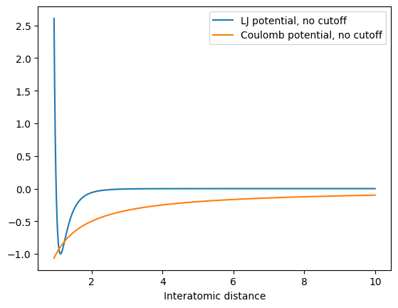

Note that the orange curve never decays close to 0 on any reasonable distance. This is especially a problem with periodic boundary conditions, where particles interact with themselves in the surrounding images, which we cannot capture with a simple cutoff. We therefore have to compute charged interactions differently.

Ewald summation¶

How can we compute electrostatic interactions with periodic boundary conditions without using a cutoff?

Approach (Ewald summation): Originally developed in 1921 to compute the Madelung constant of ionic crystals. Works for periodic systems where the unit cell is charge-neutral.

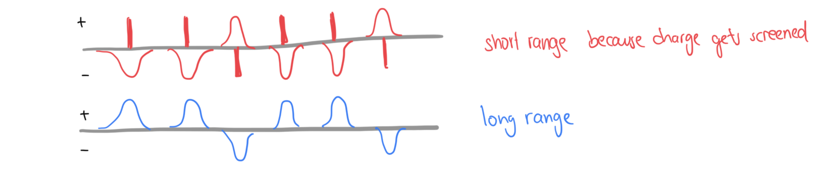
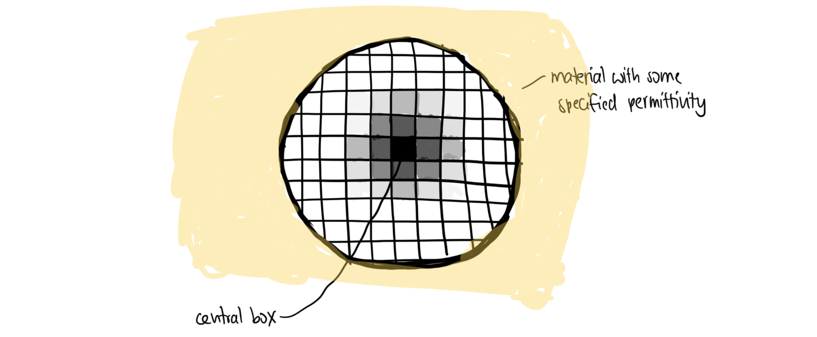
The principle is to divide the Coulomb potential into a short-range and long-range part: $V_\mathrm{Coulomb} = V_\mathrm{short-range}(\overrightarrow{R}) + V_\mathrm{long-range}(\overrightarrow{R})$

We then treat interactions with neighboring cells up to a very large cutoff, and then pretend that our system is immersed into a continuum:

Let us re-examine the Coulomb potential, including all images of the periodic boundary conditions:

$V_\mathrm{Coulomb} = \frac{1}{2} \sum_{\overrightarrow{n}}\sum_{i} \sum_{j} \frac{q_iq_j}{4\pi\epsilon_0 |\overrightarrow{r_{ij}} + \overrightarrow{n}|}$ with $i\neq j$ if $|\overrightarrow{n}|=0$

$\overrightarrow{n} = (n_xL,n_yL,n_zL)$ $|\overrightarrow{n}| = 0, 1, \sqrt{2}, \sqrt{3}, 2, ... \cdot L$

This formulation is very slow convergence, and conditionally convergent (meaning that there is a mixture of positive and negative terms, which both diverge on their own)

We thus reformulate using the following idea: $\frac{1}{r} = \textcolor{red}{\frac{f(r)}{r}}+ \textcolor{blue}{\frac{1-f(r)}{r}}$ where we choose an appropriate function $f(r)$ to get rapid conversion for both.

We assume that the neutralising charge distribution is Gaussian: $\rho_i (\overrightarrow{r}) = \frac{q_i \alpha^3}{\pi^{3/2}} e^{-\alpha^2r^2}$

The interaction with point charges + neutralising charges then becomes: $\textcolor{red}{V_\mathrm{short-range}} = \frac{1}{2} \sum_{\overrightarrow{n}}\sum_{i} \sum_{j} \frac{q_iq_j ~ \mathrm{erfc}(\alpha |\overrightarrow{r_{ij}} + \overrightarrow{n}|)}{4\pi\epsilon_0 |\overrightarrow{r_{ij}} + \overrightarrow{n}|}$

with $\mathrm{erfc}(x) = \frac{2}{\pi}\int_x^\infty e^{-t^2}\mathrm{d}t$ ... which is our $f(r)$ from above.

This summation (which is the short term, real space summation) converges very rapidly and can be considered negligible after some cutoff:

Narrow Gaussian (large $\alpha$ ): Faster convergence
Wide Gaussian (small $\alpha$ ): Slower convergence
$\alpha$ should always be chosen such that the only term in the series are those for $|\overrightarrow{n}| =0$

Contribution from second charge distribution (which is the long-term, reciprocal space summation) converges very rapidly in Fourier space: $\textcolor{blue}{V_\mathrm{long-range}} = \frac{1}{2} \sum_{k\neq 0}\sum_{i} \sum_{j} \frac{1}{\pi L^3}\frac{q_iq_j }{4\pi\epsilon_0} \frac{4\pi^2}{k^2} e^{-\frac{k^2}{4\alpha^2}}\mathrm{cos}(\overrightarrow{k}\overrightarrow{r_{ij}})$ with the reciprocal vectors $\overrightarrow{k} = \frac{2\pi\overrightarrow{n}}{L}$

Narrow Gaussian (large $\alpha$ ): Slower convergence
Wide Gaussian (small $\alpha$ ): Faster convergence
Default: $\alpha \simeq 5/L$ with 100-200 reciprocal vectors $\overrightarrow{k}$

There is also a correction term for the interaction of each Gaussian with itself in real-space:

$V_\mathrm{corr} = -\frac{\alpha}{\sqrt{\pi}} \sum_{k\neq 0} \frac{q_k^2}{4\pi\epsilon_0}$

If surrounding medium is vacuum, then even another correction term is needed (for a conducting medium with infinite relative permittivity, no further correction is needed).

Using the equations above, we can now compute Coulomb interactions with periodic boundary conditions. The Ewald sum is really accurate, but scales with $N^2$

Faster: Particle-mesh Ewald (PME) which scales with $N$ log $N$ :

Real space (“particle” part of PME) as above, but Fourier space (“mesh” part of PME) uses the fast Fourier transform instead.
Since FFT only works with discrete data, we have to fit our atomic point charges on continuous coordinates to a grid-based charge distribution.