Interatomic potentials

$n$-body potentials¶

Classic approach (as approximation of true, quantum-mechanical energy)}

$E_\mathrm{pot}\{\overrightarrow{r}_I\} = V_0$ $+ \sum_I V_1(\overrightarrow{r}_I)$ $+ \sum_{I,J} V_2(\overrightarrow{r}_I,\overrightarrow{r}_J)$ $+ \sum_{I,J, K} V_3(\overrightarrow{r}_I,\overrightarrow{r}_J,\overrightarrow{r}_K)$ $+ \sum_{I,J, K,L} V_4(\overrightarrow{r}_I,\overrightarrow{r}_J,\overrightarrow{r}_K,\overrightarrow{r}_L)$ + ...

The best choice of potential depends on the state of the system (gas, liquid, solid), and the type of bonds (covalent bonds, non-bonded interactions, crystal/metal lattices)

For non-bonded interactions, a two-body potential is usually a good description already. For bonded interaction, many more terms are needed!

Two-body potentials $V_2(R)$¶

Noble gases:

• Lennard-Jones potential 1924: $V_2(R) = 4\epsilon\left[\left(\frac{\sigma}{R}\right)^{12} - \left(\frac{\sigma}{R}\right)^{6}\right]$ to model noble gases.

• Buckingham potential 1938: $V_2(R) = Ae^{-BR} - \frac{C}{R^6}$ allows for a more flexible form than Lennard-Jones

Covalent (only diatomic) bonds:

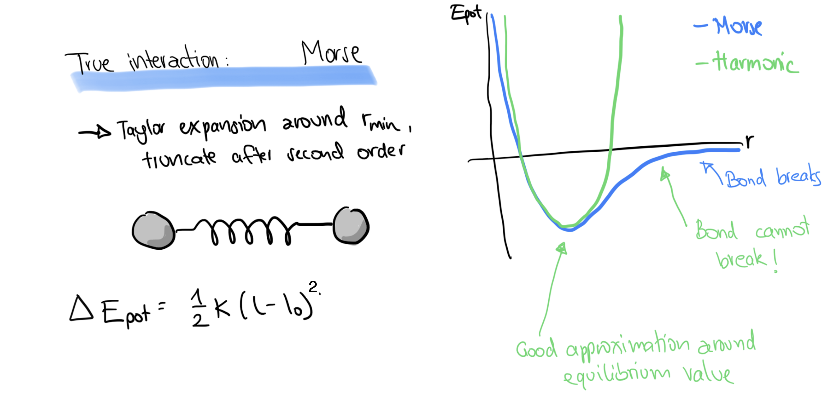
• Morse potential 1929: $V_2(R) = D_e\left[\left(1-e^{-\alpha(R-R_c)}\right)^{2} -1 \right]$ describes many diatomic systems well. Minimum at $R_c$ with the potential energy $-D_e$

Solid state:

• Stillinger-Weber potential 1985: $V_2(R) = A\epsilon\left[B\left(\frac{\sigma}{R}\right)^{p} - \left(\frac{\sigma}{R}\right)^{q}\right] e^{\frac{\sigma}{R-a\sigma}}$ and $V_3(R_{IJ},R_{IK},\theta_{IJK}) = \lambda \epsilon (cos\theta_{IJK} - cos\theta_{0})^2 e^{\frac{\gamma\sigma}{R_{IJ}-a\sigma}} e^{\frac{\gamma\sigma}{R_{IK}-a\sigma}}$ to model solid and liquid phases of Si, GaN, 2D materials, etc.

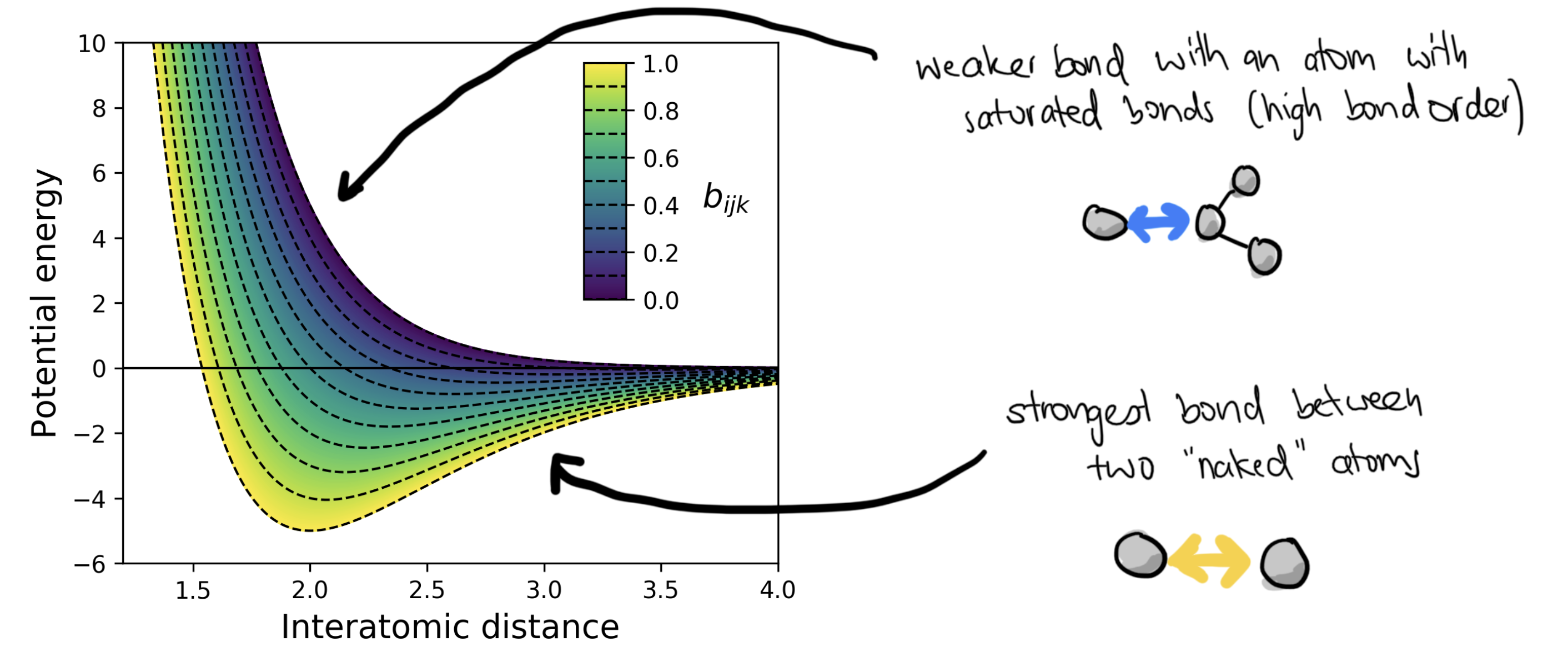
• Tersoff’s bond-order potential 1988: $V_2(R_{IJ}) = f_c(R_{IJ})[f_r(R_{IJ} + b_{IJ}f_a(R_{IJ})]$ which is a two-body potential where the attractive part is modulated by the bond order $b_{IJ}$ which depends on $\theta_{IJK}$

Molecular mechanics¶

Molecular systems (with a bent toward organic molecules in fluid phases)

• Potential has bonded and non-bonded interactions

• Atoms have vdW radii, partial charges and possibly polarizabilities

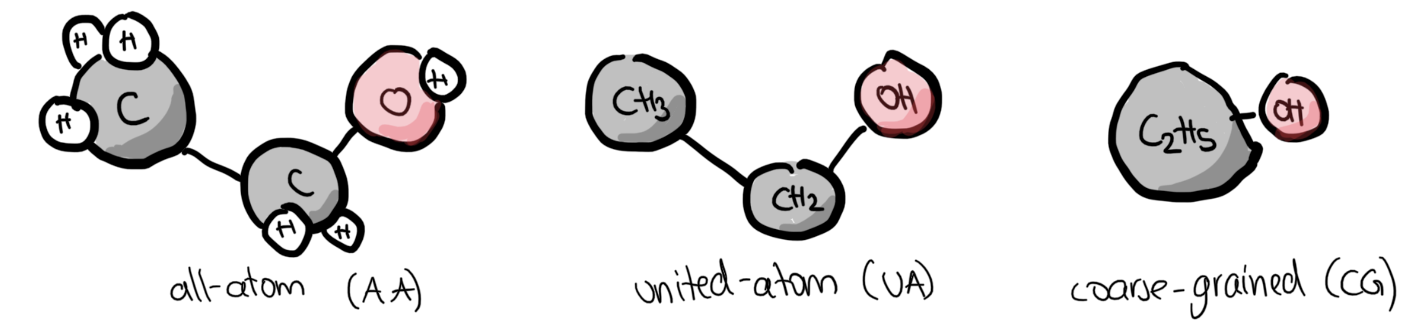
• Molecules can be treated in an all-atom, united-atom (implicit hydrogen) or coarse-grained (multiple atom form a bead) fashion. Parts of the simulation can also be at the QM-level (QM-MM hybrid approach)

e.g. OPLS-AA 1996: The potential is a sum of bonded and non-bonded energy terms: $V = V_\mathrm{bonded} + V_\mathrm{non-bonded}$

Bonded terms:

• Bond-term $V_\mathrm{bond} = \sum_\mathrm{bonds~IJ} K_R(I,J)[R_{IJ} - R_{0,IJ}]^2$

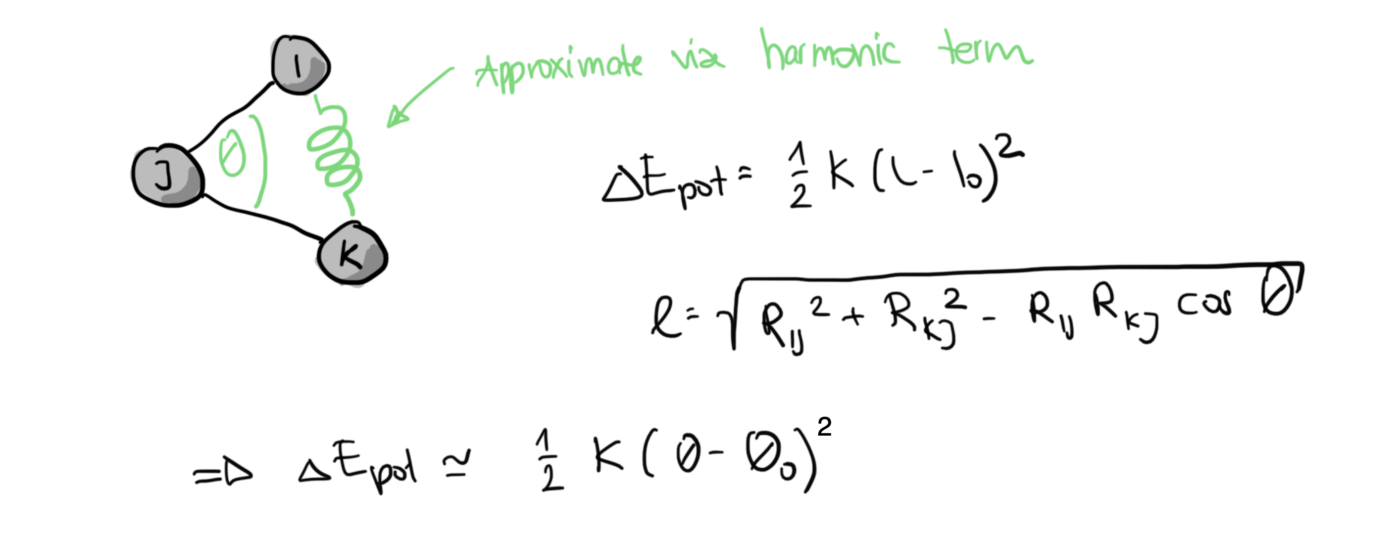
• Angle-term $V_\mathrm{angle} = \sum_\mathrm{angles~IJK} K_\theta(I,J,K)[\theta_{IJK} - \theta_{0,IJK}]^2$

• Dihedral-term $V_\mathrm{dihedral} = \sum_\mathrm{dihedrals~IJKL} \frac{K_1}{2}[1 + cos(\phi_{IJKL} - \phi_1)] + \frac{K_2}{2}[1 - cos(2\phi_{IJKL} - \phi_2)] + \frac{K_3}{2}[1 + cos(3\phi_{IJKL} - \phi_3)] + \frac{K_4}{2}[1 - cos(4\phi_{IJKL} - \phi_4)]$

Non-Bonded terms: Combined vdW and charge interactions: $V_\mathrm{non-bonded} = \sum_{I>J} f_{IJ} \left( \frac{A_{IJ}}{R_{IJ}^{12}} - \frac{C_{IJ}}{R_{IJ}^{6}} + \frac{q_I q_J e^2}{4\pi\epsilon R_{IJ}} \right)$ with combining rules $A_{IJ}=\sqrt{A_{ii}A_{jj}}$ and $C_{IJ}=\sqrt{C_{ii}C_{jj}}$ and $f_{IJ}$ is 1/0.5/0 if I and J are more than/exactly/less than 3 bonds apart.

Two-body terms in molecular potentials (= bonds)¶

Three-body terms in molecular potentials (= angles)¶

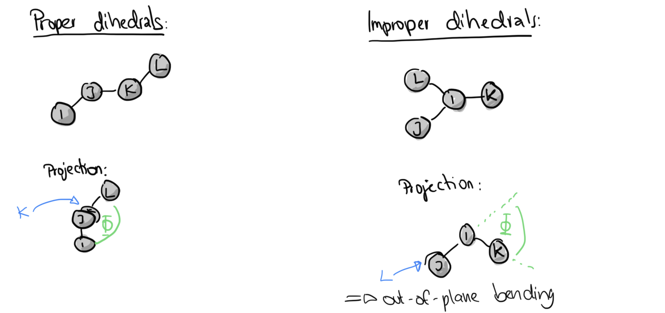
Four-body terms in molecular potentials (= dihredral angles)¶

In the following, we will generate a trajectory for ethane, and try to reverse-engineer the potential:

From the distribution of bond lengths, we can compute the potential of mean force, which should approximately recreate the potential we used to make the trajectory (namely the bonded term $E_\mathrm{bond} = \frac{1}{2}{K}(r-r_\mathrm{eq})^2$ with $r_\mathrm{eq} = 0.15380$nm and $K=1945727.36$ kJ/mol $\cdot$ nm$^2$, values taken from the XML file above).

The potential of mean force is defined as

where $p(x)$ if the probability (the histogram) we calculated above.

Let us also analyze the H-C-C-H torsion. To do so, we only need to change md.core.topologyobjects.Bond to md.core.topologyobjects.Dihedral and use the correct indices.

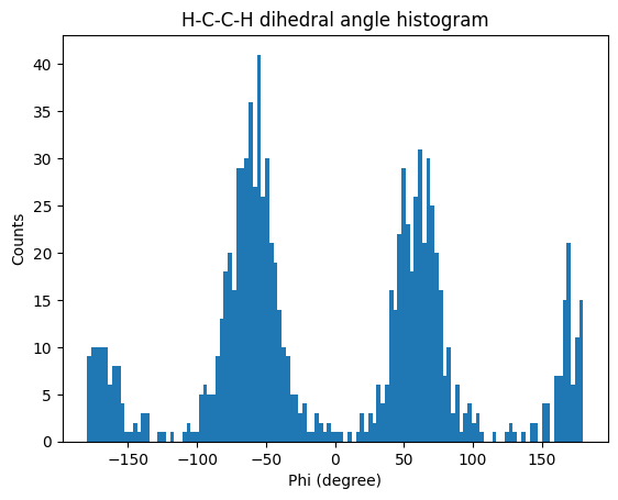
To compare with the $E_\mathrm{dihedral}$ term, we have to remember that there are nine terms that change when we turn along the C-C bond (below, we only followed how a single bond changed, and thus only one term in the energy was affected).

• H11-C1-C2-H21

• H11-C1-C2-H22

• H11-C1-C2-H23

• H12-C1-C2-H21

• H12-C1-C2-H22

• H12-C1-C2-H23

• H13-C1-C2-H21

• H13-C1-C2-H22

• H13-C1-C2-H23

We therefore multiply a single $E_\mathrm{dihedral}$ term by 9 to get a good comparison:

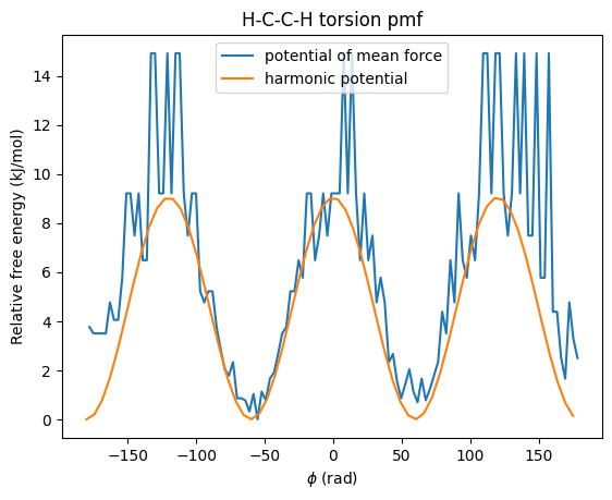
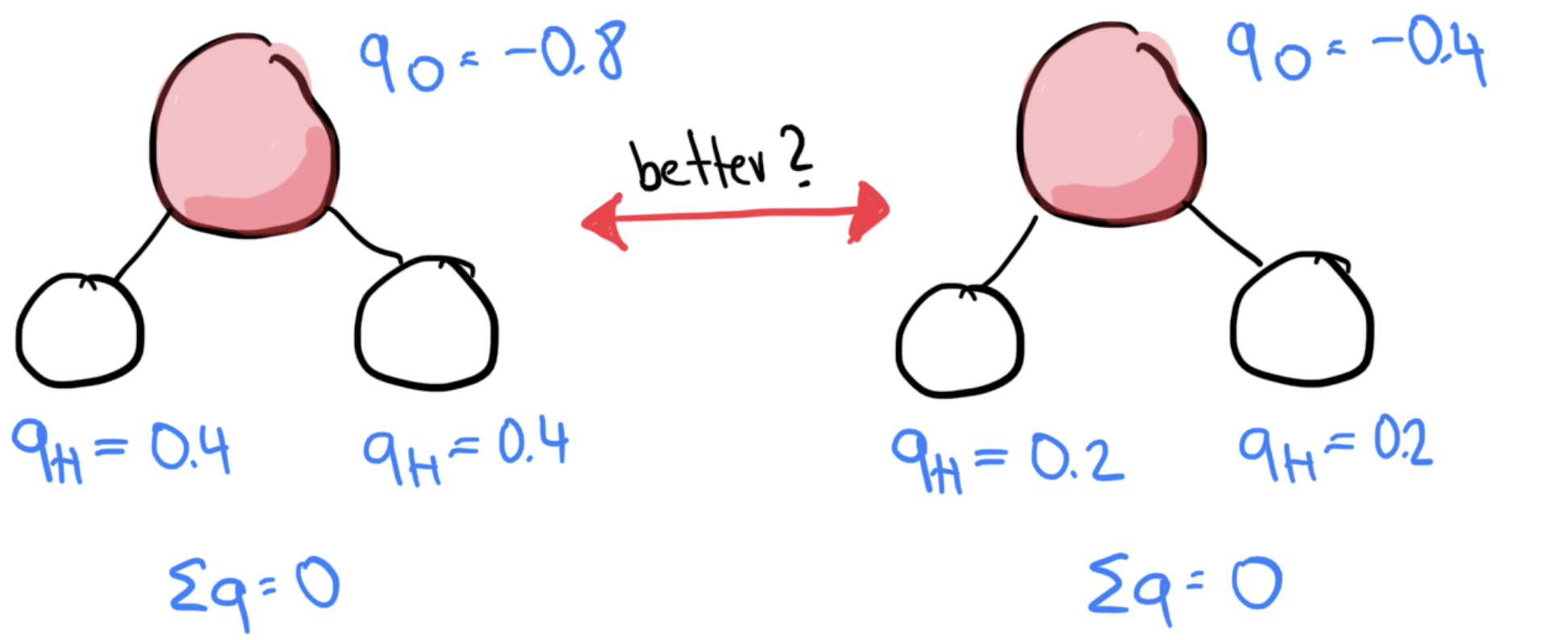
Partial charges¶

There is no physical quantity such as an “atomic charge”, there are therefore many valid schemes to assign partial charges, e.g. (among many others)

• Formal charges

• Restrained fit to the electrostatic potential (RESP)

• Mulliken charges

• Bader charges

Polarizability¶

Reactive (molecular) force fields¶

For LJ, Buckingham, Morse-type FFs, reactivity is not a problem:

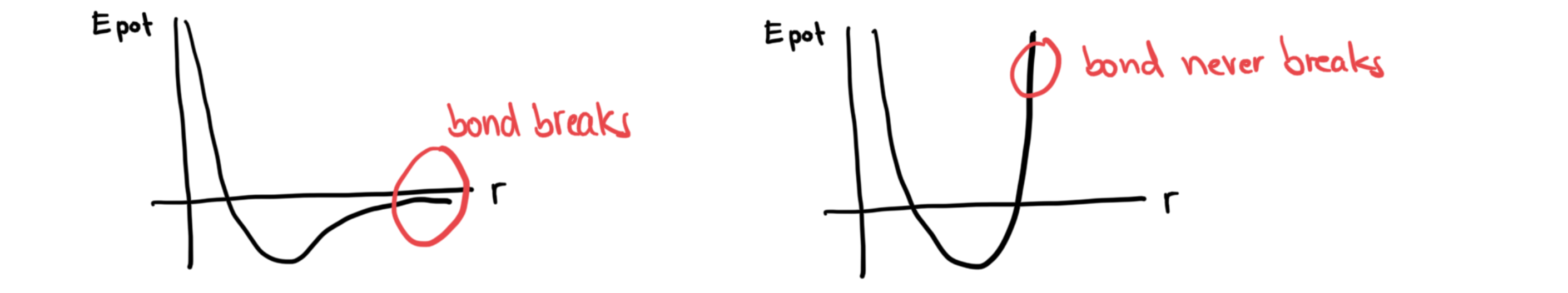
But for molecular force fields, because we change the Morse term to an harmonic term, all bonds become unbreakable

Possible solutions:

• General reactive force fields based on bond-order potentials, for example ReaxFF

• Force fields without enforced functional form, e.g. from machine learning

• For simple cases, e.g. protonation reactions, one can also work with ghost atoms

A potential for water¶

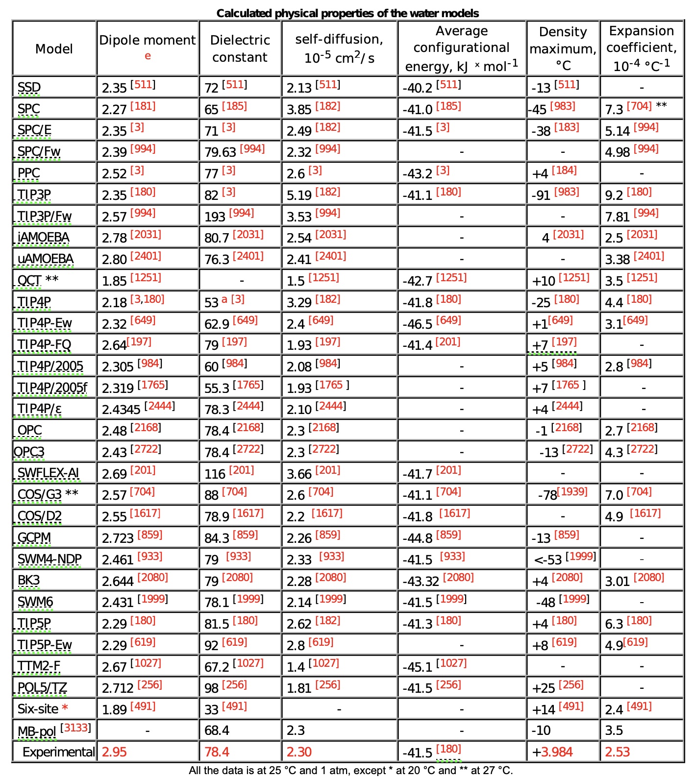
There are nearly 50 water potentials reported in literature, which follow the general forms

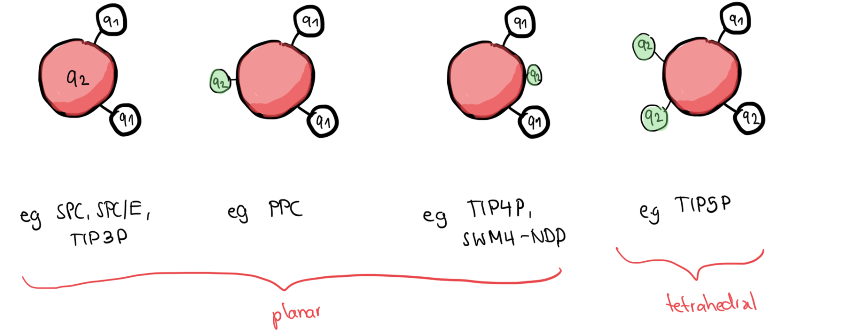
Yet, none of them capture all the properties of water well:

(from https://water.lsbu.ac.uk/water/water_models.html)